12.1.2 DCGAN Art

Overview

Deep Convolutional Generative Adversarial Networks (DCGANs) were introduced by Radford et al. in 2015. They apply convolutional neural network architectures to the GAN framework, producing images with coherent spatial structure where fully-connected GANs produced noise.

In this exercise you will generate abstract art with a pre-trained DCGAN, explore the learned latent space through interpolation, and (optionally) train the network from scratch on a real dataset of African fabric patterns. The narrative arc: in early modules you wrote algorithms to generate patterns by hand; here, you teach a neural network to learn and generate similar patterns autonomously.

Learning objectives

1. Understand why convolutional architectures improve image generation over fully-connected networks.
2. Analyse the Generator and Discriminator components of a DCGAN.
3. Generate novel abstract art by sampling from the learned latent space.
4. Explore latent-space interpolation to create smooth transitions between generated images.

Quick start — see it in action

Load the pre-trained generator and produce four random art pieces.

import torch
from dcgan_model import Generator, LATENT_DIM
import matplotlib.pyplot as plt

# Load pre-trained generator
generator = Generator()
generator.load_state_dict(torch.load('exercise3_generator.pth', map_location='cpu'))
generator.eval()

# Generate 4 random art pieces
z = torch.randn(4, LATENT_DIM, 1, 1)
with torch.no_grad():
    images = generator(z)

# Display the generated art
images = (images + 1) / 2  # Convert from [-1, 1] to [0, 1]
fig, axes = plt.subplots(1, 4, figsize=(12, 3))
for i, ax in enumerate(axes):
    ax.imshow(images[i].permute(1, 2, 0).numpy())
    ax.axis('off')
plt.savefig('quick_start_output.png', dpi=150)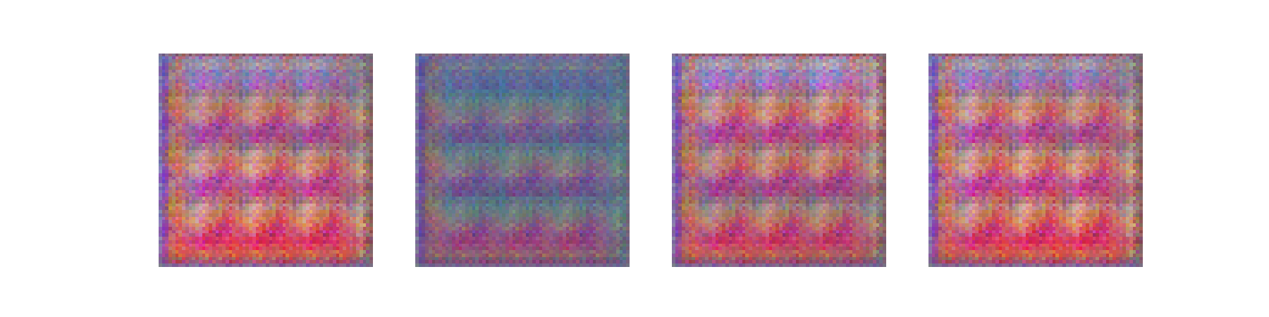

The generator transforms 100-dimensional random noise vectors into 64×64 pixel RGB images. The patterns exhibit smooth gradients, geometric shapes, and colour harmonies learned from training data.

Core concepts

Concept 1 — From fully-connected to convolutional

Traditional GANs using fully-connected layers struggle to generate coherent images because they treat each pixel independently. Consider a 64×64 RGB image: that is 12,288 values the network must generate without any understanding of spatial relationships.

Convolutional Neural Networks (CNNs) solve this by exploiting the spatial structure of images. Three key properties make CNNs effective for image generation:

1. Local connectivity — each neuron connects to a small region (receptive field), learning local patterns.
2. Weight sharing — the same filter is applied across the entire image, learning translation-invariant features.
3. Hierarchical features — lower layers detect edges and textures; higher layers combine these into complex patterns.

DCGANs apply these principles to both the generator (which uses transposed convolutions to upsample) and the discriminator (which uses standard convolutions to downsample).

Concept 2 — DCGAN architecture

A DCGAN consists of two competing networks: a Generator that creates images from noise, and a Discriminator that distinguishes real images from generated ones.

class Generator(nn.Module):
    def __init__(self, latent_dim=100, img_channels=3, feature_maps=64):
        super().__init__()
        self.network = nn.Sequential(
            # Input: 100 × 1 × 1 latent vector
            # Layer 1: 100 → 4 × 4 × 512
            nn.ConvTranspose2d(latent_dim, feature_maps * 8, 4, 1, 0),
            nn.BatchNorm2d(feature_maps * 8),
            nn.ReLU(True),

            # Layer 2: 4 × 4 × 512 → 8 × 8 × 256
            nn.ConvTranspose2d(feature_maps * 8, feature_maps * 4, 4, 2, 1),
            nn.BatchNorm2d(feature_maps * 4),
            nn.ReLU(True),

            # Layer 3: 8 × 8 × 256 → 16 × 16 × 128
            nn.ConvTranspose2d(feature_maps * 4, feature_maps * 2, 4, 2, 1),
            nn.BatchNorm2d(feature_maps * 2),
            nn.ReLU(True),

            # Layer 4: 16 × 16 × 128 → 32 × 32 × 64
            nn.ConvTranspose2d(feature_maps * 2, feature_maps, 4, 2, 1),
            nn.BatchNorm2d(feature_maps),
            nn.ReLU(True),

            # Layer 5: 32 × 32 × 64 → 64 × 64 × 3
            nn.ConvTranspose2d(feature_maps, img_channels, 4, 2, 1),
            nn.Tanh()  # Output in [-1, 1]
        )

• The first layer expands the latent vector to a 4×4 spatial grid with 512 channels.
• Each subsequent layer doubles the spatial resolution while halving the channels.
• The final layer produces a 3-channel RGB image with Tanh activation.

The discriminator mirrors the generator, using strided convolutions to downsample from 64×64 to a single scalar.

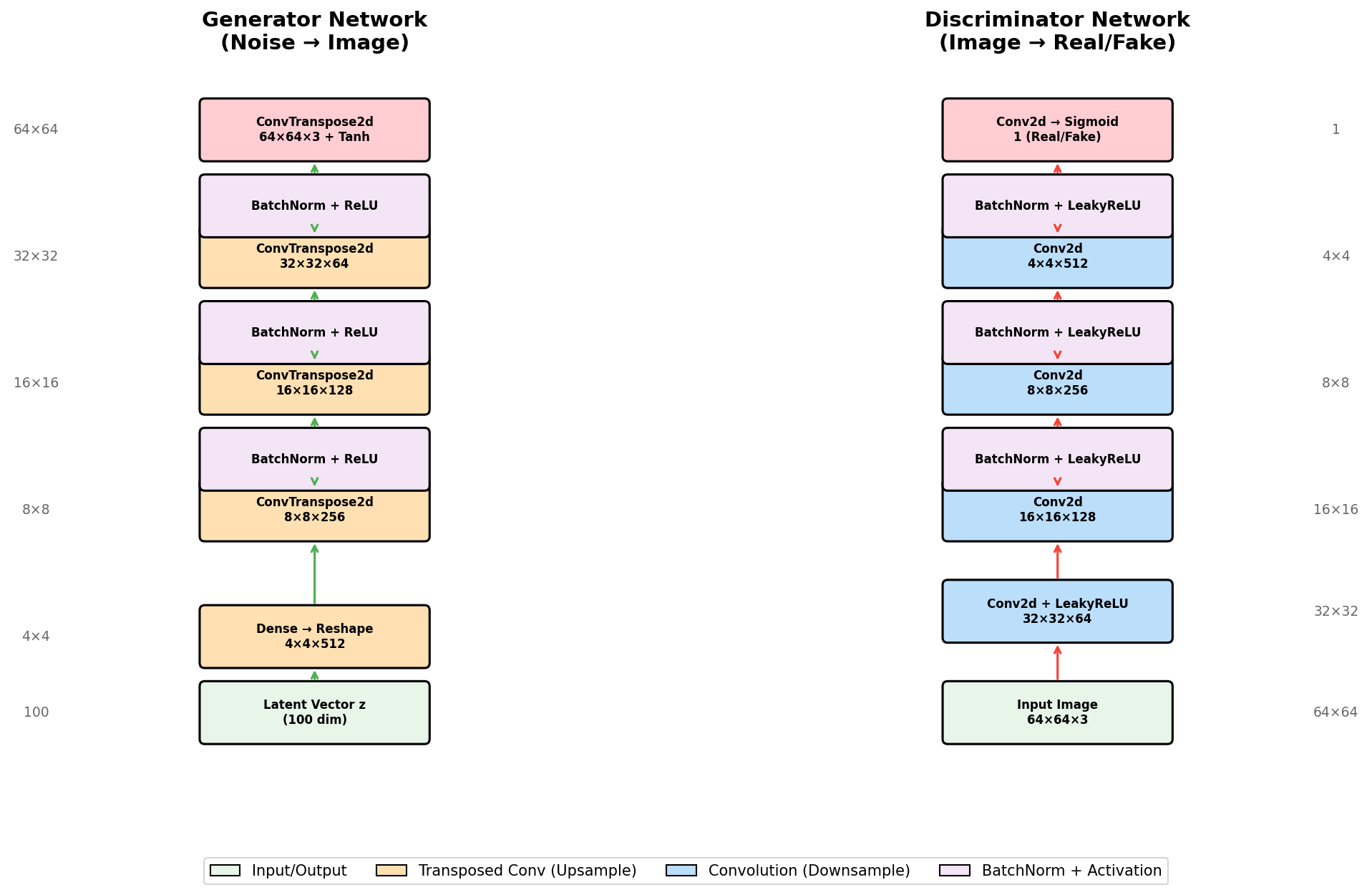
Architectural guidelines from the DCGAN paper:

1. Replace pooling with strided convolutions (discriminator) and transposed convolutions (generator).
2. Use Batch Normalisation in both networks (except discriminator input and generator output).
3. Use ReLU in the generator (except the output, which uses Tanh).
4. Use LeakyReLU in the discriminator to prevent sparse gradients.

Concept 3 — Latent space and art generation

The latent space is the 100-dimensional space from which the generator samples input vectors. Each point in this space corresponds to a unique generated image; nearby points produce visually similar images.

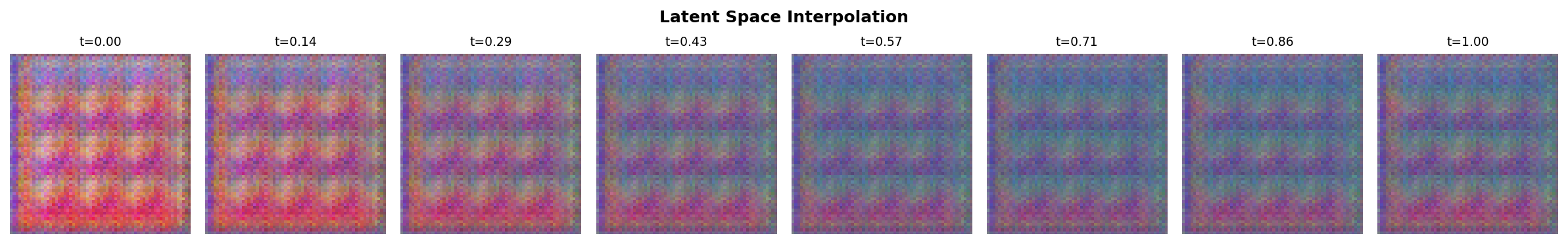
This property enables creative applications. Interpolation: by smoothly transitioning between two latent vectors, we morph one image into another.

def interpolate(z1, z2, steps=10):
    """Generate images along a path between two latent points."""
    images = []
    for t in range(steps):
        alpha = t / (steps - 1)
        z = (1 - alpha) * z1 + alpha * z2  # Linear interpolation
        z = z.view(1, 100, 1, 1)
        img = generator(z)
        images.append(img)
    return images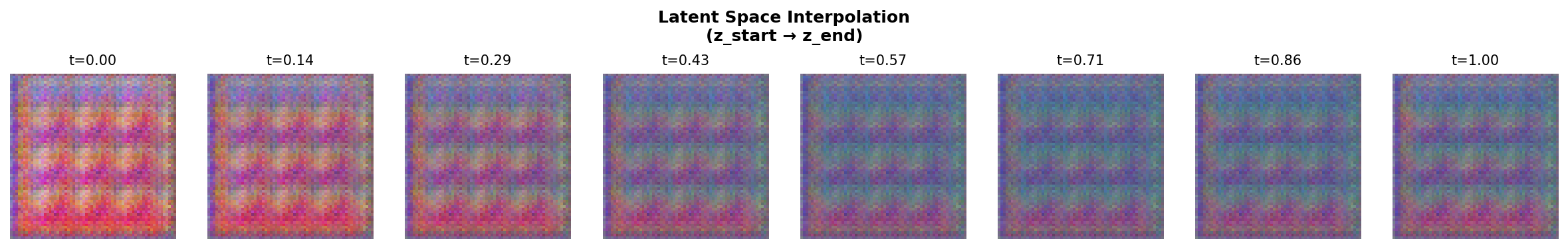

Exercises

EXECUTE I.

Observe DCGAN generation

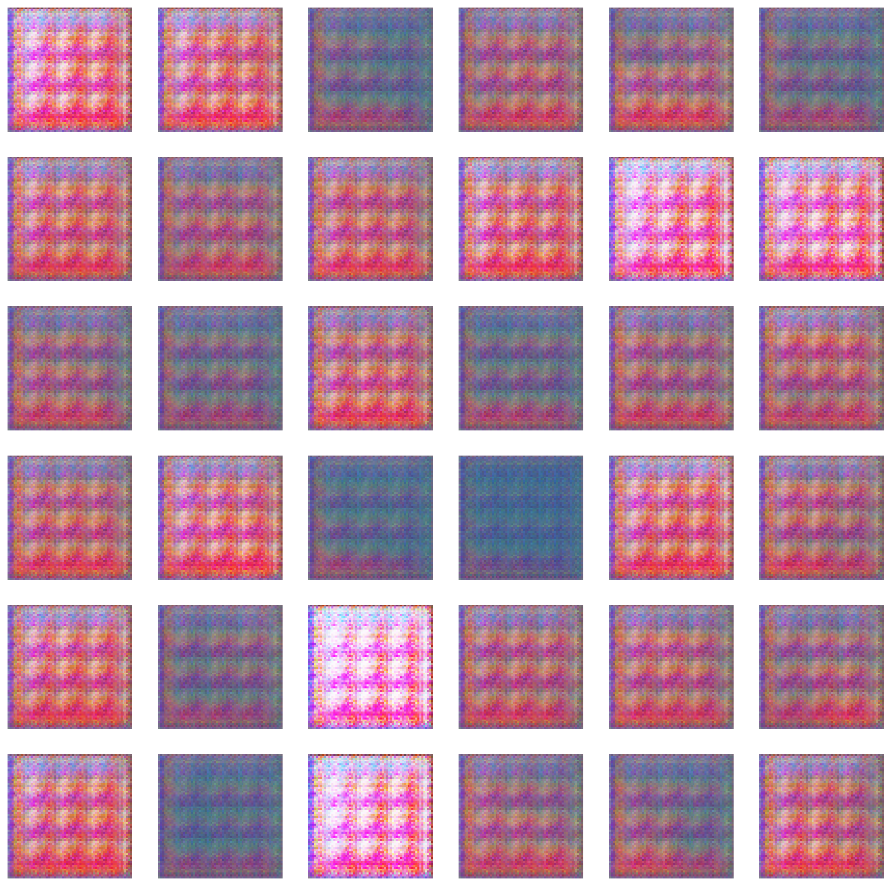
Run the pre-trained generator to see how DCGANs create abstract art from random noise vectors. The script produces a 4×4 grid of unique patterns.

exercise1_observe.py

bash Copy

python exercise1_observe.py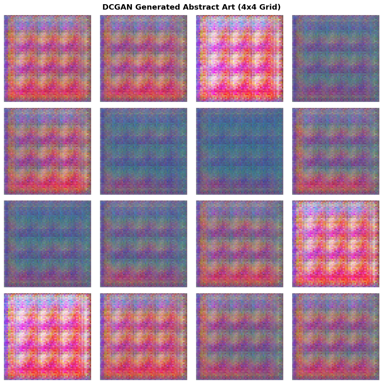

Reflection

1. How does the latent vector size (100 dimensions) affect the diversity of generated art?
2. What common visual patterns do you observe across samples?
3. Why does the generator use Tanh activation in the output layer?

Discussion

1. The 100-dimensional latent space provides enough capacity for the generator to learn diverse patterns. Smaller dimensions (like 50) would limit variety; larger dimensions (like 200) would increase training difficulty without much benefit.
2. You should observe smooth colour gradients, geometric shapes (circles, stripes), and harmonious palettes. These reflect the procedural patterns in the training dataset.
3. Tanh outputs values in [-1, 1], matching the normalised range of training images. This bounded output prevents extreme pixel values and ensures stable gradients during training.

MODIFY II.

Explore parameters and interpolation

Experiment with generation parameters: larger grids, more interpolation steps, and different random seeds.

exercise2_explore.py

The script demonstrates two explorations:

1. Larger grid — generates a 6×6 grid (36 samples) to see more variation.
2. Latent interpolation — creates smooth transitions between two random latent vectors.

Try these modifications

• Change the random seed to generate different sample sets.
• Modify grid size (try 8×8 or 10×10).
• Increase interpolation steps to 16 or 32 for smoother transitions.
• Compare linear interpolation at different points in latent space.

Tips

• Memory — when generating many images, the script uses torch.no_grad() to save memory.
• Interpolation smoothness — more steps create smoother transitions but take longer to generate.
• Random seeds — different seeds explore different regions of the latent space.

TRAIN III.

Train on African fabric patterns

Train a DCGAN from scratch on African fabric patterns from Kaggle. Demonstrates the complete training process from dataset preparation through 100 epochs of adversarial training.

Time commitment

• Dataset setup: 5–10 min (one-time)
• Training: 20–30 min on GPU, 60–90 min on CPU
• Observation: 10 min

Dataset setup — download and preprocess

Use the African Fabric dataset from Kaggle (~1,059 images, vibrant textile patterns).

Step 1 — Download: visit kaggle.com/datasets/mikuns/african-fabric, download, and extract to african_fabric_dataset/ inside the lesson directory.

Step 2 — Preprocess — run preprocess_african_fabric.py to resize to 64×64, convert to RGB, and save to african_fabric_processed/.

preprocess_african_fabric.py

Training configuration & execution

Hyperparameters:

• Epochs: 100
• Batch size: 64
• Learning rate: 0.0002 (both networks)
• Optimiser: Adam, β₁=0.5, β₂=0.999
• Loss: Binary Cross-Entropy (BCE)
• Dataset: 1,059 fabric patterns (64×64 RGB)

exercise3_train.py

bash Copy

python exercise3_train.py

The script will:

1. Load the dataset from african_fabric_processed/.
2. Initialise the Generator and Discriminator.
3. Train for 100 epochs with per-epoch progress updates.
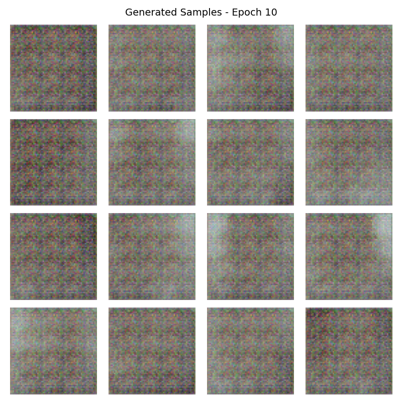
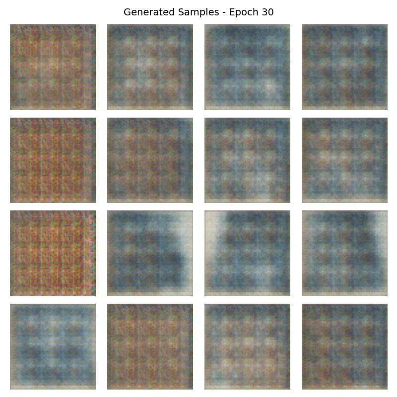
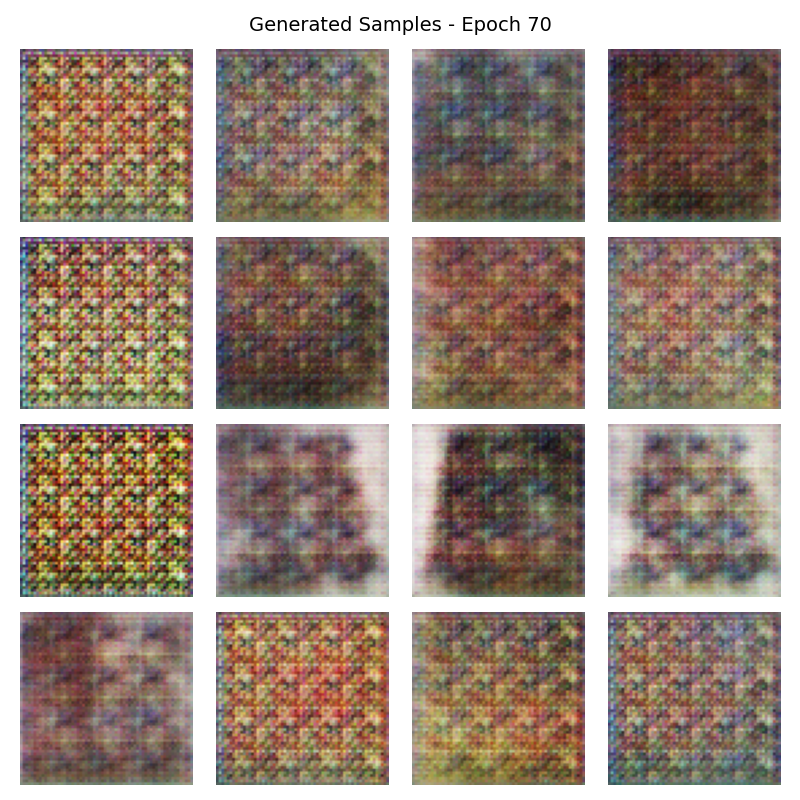
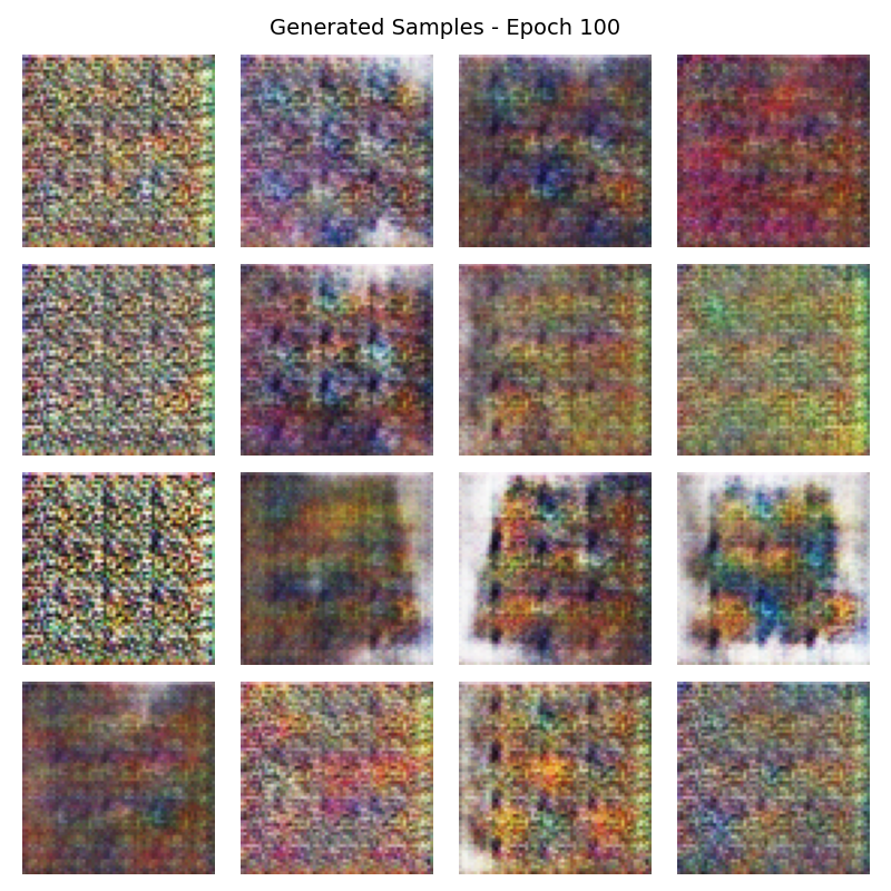
4. Save checkpoints at epochs 10, 30, 50, 70, and 100.
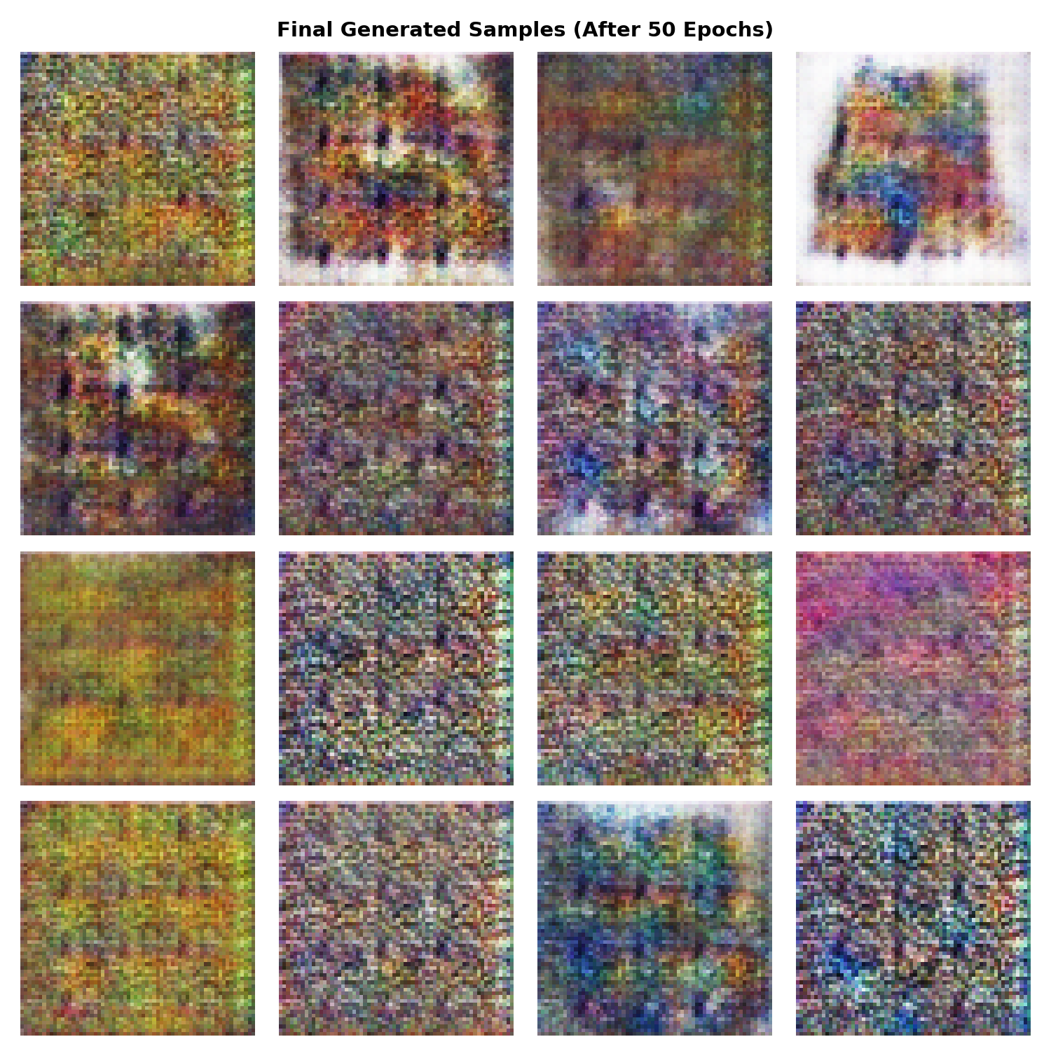
5. Save the final trained model as exercise3_generator.pth.

What to observe during training

• Loss oscillation — both G and D losses fluctuate significantly (this is normal).
• Occasional spikes — sudden jumps are expected in GAN training.
• No clear convergence — unlike supervised learning, GAN losses don’t smoothly decrease to zero.

Training results — 100 epochs of learning

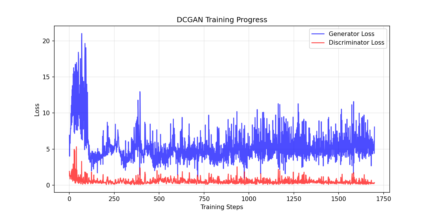
Watch the generator’s visual progression across checkpoints:

Implementation note

Challenge extensions

Summary

Common pitfalls

• Mode collapse — generator produces limited variety. Adjust learning rates or use minibatch discrimination.
• Checkerboard artifacts — caused by transposed convolutions. Use resize-convolution instead.
• Training instability — monitor both losses; if one dominates, adjust learning rates.
• Wrong output range — forgetting Tanh or input normalisation causes divergence.
• Dimension mismatches — latent vectors must have shape (batch, latent_dim, 1, 1), not (batch, latent_dim).

References

- [1] Radford, A., Metz, L. & Chintala, S. (2015). Unsupervised Representation Learning with Deep Convolutional Generative Adversarial Networks. arXiv preprint. arxiv:1511.06434
- [2] Goodfellow, I., Pouget-Abadie, J., Mirza, M., Xu, B., Warde-Farley, D., Ozair, S., Courville, A. & Bengio, Y. (2014). Generative Adversarial Nets. Advances in Neural Information Processing Systems, 27.
- [3] Goodfellow, I., Bengio, Y. & Courville, A. (2016). Deep Learning. MIT Press. ISBN 978-0-262-03561-3.
- [4] LeCun, Y., Bengio, Y. & Hinton, G. (2015). Deep learning. Nature, 521(7553), 436–444.
- [5] Ioffe, S. & Szegedy, C. (2015). Batch Normalization. arXiv preprint. arxiv:1502.03167
- [6] Kingma, D. P. & Welling, M. (2014). Auto-Encoding Variational Bayes. arXiv preprint. arxiv:1312.6114
- [7] Odena, A., Dumoulin, V. & Olah, C. (2016). Deconvolution and Checkerboard Artifacts. Distill. distill.pub/2016/deconv-checkerboard/
- [8] PyTorch Contributors. (2024). DCGAN Tutorial. pytorch.org/tutorials/beginner/dcgan_faces_tutorial.html