9.1.1 Perceptron from Scratch

Big question

What is the simplest machine that can learn to classify data? Frank Rosenblatt’s 1958 perceptron is the answer — and it is so simple you can implement it in thirty lines of NumPy. Three operations: multiply inputs by weights, sum the products, threshold the result. The novel addition was a learning rule: after every wrong prediction, nudge each weight in the direction that would have produced the right answer. Run this loop on linearly separable data and the weights converge to a hyperplane that splits the two classes [1, 2]. The same weight-update logic, generalised through calculus, runs inside every modern neural network with billions of parameters.

Learning objectives

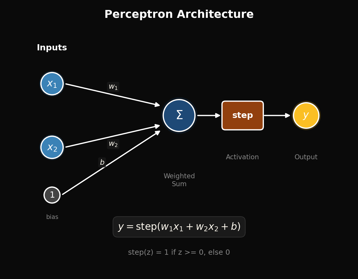
1. State the perceptron architecture: weighted sum, bias, step activation.
2. Implement the forward pass with np.dot and a step function.
3. Apply the perceptron learning rule: w ← w + lr × (y_true − y_pred) × x.
4. Visualise the learned decision boundary as a line in 2D feature space.
5. Recognise the XOR limitation that motivated multi-layer networks.

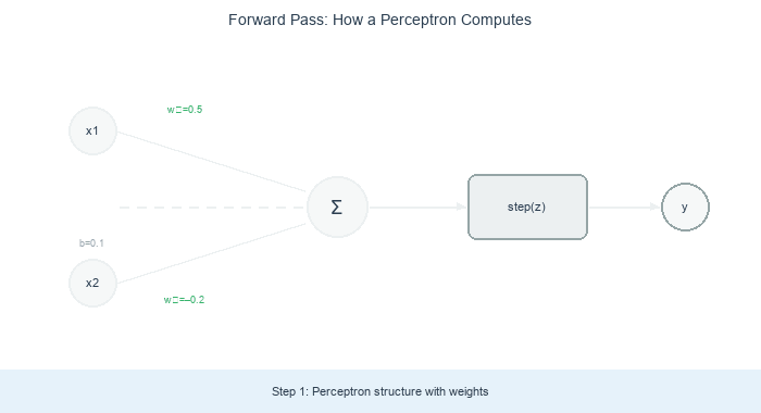
Part 1 — Architecture of a perceptron

A perceptron takes n numeric inputs (x₁, …, xₙ), multiplies each by a learned weight wᵢ, sums the products with a bias term b, and applies a step function:

def forward(self, x):
    z = np.dot(self.weights, x) + self.bias
    return 1 if z >= 0 else 0

That is the entire forward pass. The weighted sum is a single dot product; the step function is one if statement. The “neural” feel comes from analogy with McCulloch and Pitts’s 1943 biological neuron model: dendrites collect weighted inputs, the cell body integrates, the axon fires (1) when the total exceeds a threshold [3].

Part 2 — The forward pass on real data

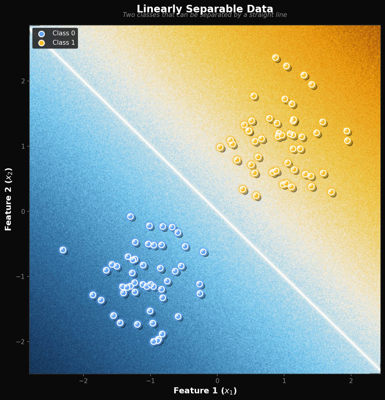
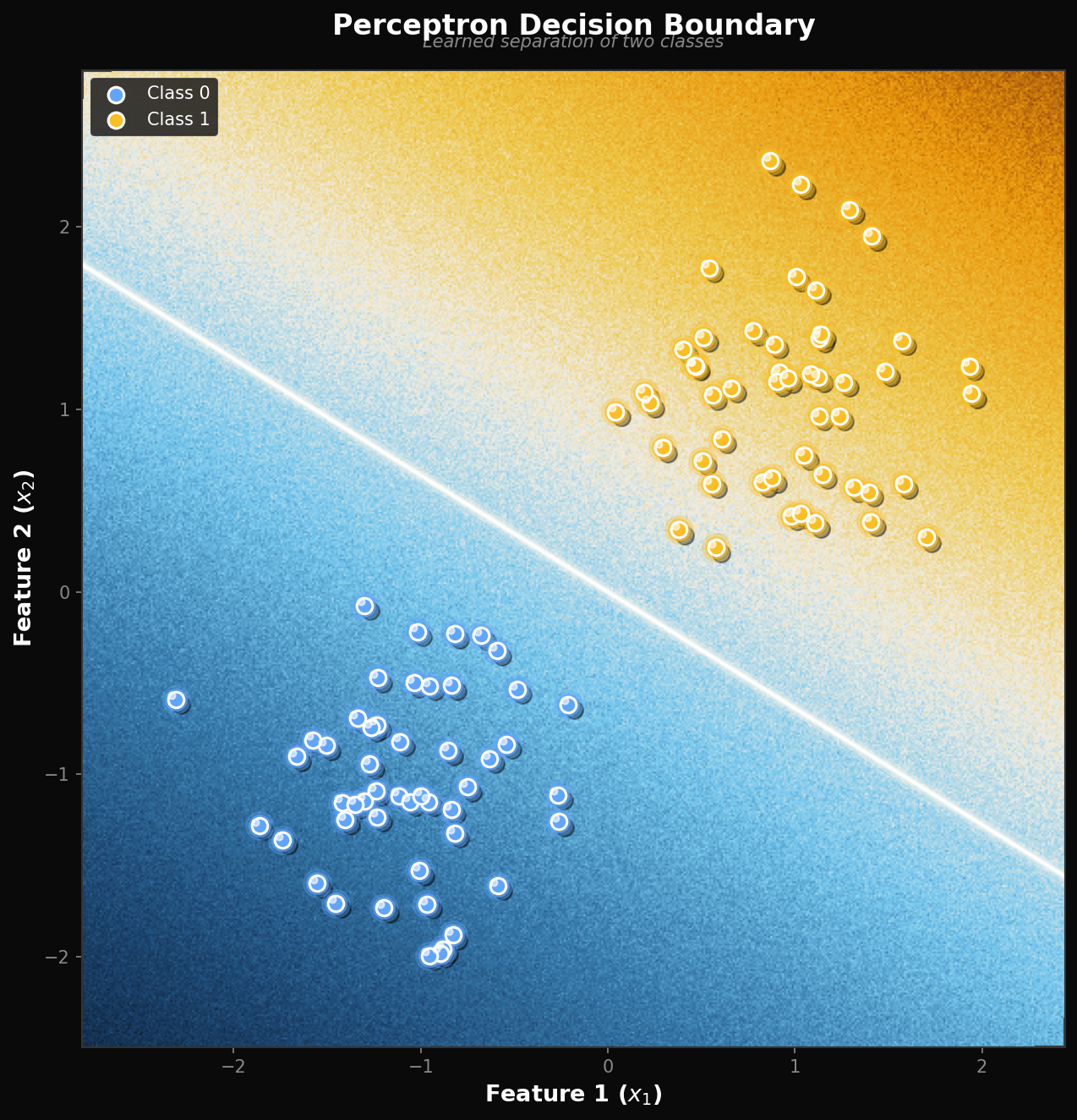
A trained perceptron’s decision rule is simple geometry: draw a line through the feature space defined by w₁ x₁ + w₂ x₂ + b = 0. Points on one side score positive (class 1); points on the other side score negative (class 0).

For a separable two-class problem (the classic “linearly separable” setup), there is at least one line that perfectly splits the classes. The perceptron learning rule promises to find it.

Part 3 — The learning rule

Rosenblatt’s 1958 weight-update rule is one line:

def update(self, x, y_true, lr=0.1):
    y_pred = self.forward(x)
    error = y_true - y_pred
    self.weights += lr * error * x
    self.bias    += lr * error

• If the prediction is correct, error = 0 and nothing changes.
• If the perceptron missed, error is ±1 and weights are pushed in the direction that would have produced the correct sign.
• The learning rate lr scales the size of each update.

Novikoff’s theorem (1962) proves this rule converges to a separating hyperplane in finite steps if one exists. The number of updates is bounded by (R/γ)² where R is the data radius and γ the margin [4].

Synthesis project

import numpy as np
import matplotlib.pyplot as plt

class Perceptron:
    def __init__(self, n_in):
        self.w = np.zeros(n_in)
        self.b = 0.0

    def forward(self, x):
        return 1 if np.dot(self.w, x) + self.b >= 0 else 0

    def update(self, x, y, lr=0.1):
        pred = self.forward(x)
        err = y - pred
        self.w += lr * err * x
        self.b += lr * err

X = np.array([[0, 0], [0, 1], [1, 0], [1, 1]], dtype=float)
y = np.array([0, 1, 1, 0])

p = Perceptron(2)
# TODO: train for 1000 epochs, shuffling each epoch.
# TODO: plot data points and the (failed) decision line.

Downloads

References