10.2.2 Boids in TouchDesigner — Physics in CHOPs, Rendering in Instances

Big Question — how do you scale a 50-agent Python sim to 5,000 agents at 60 fps?

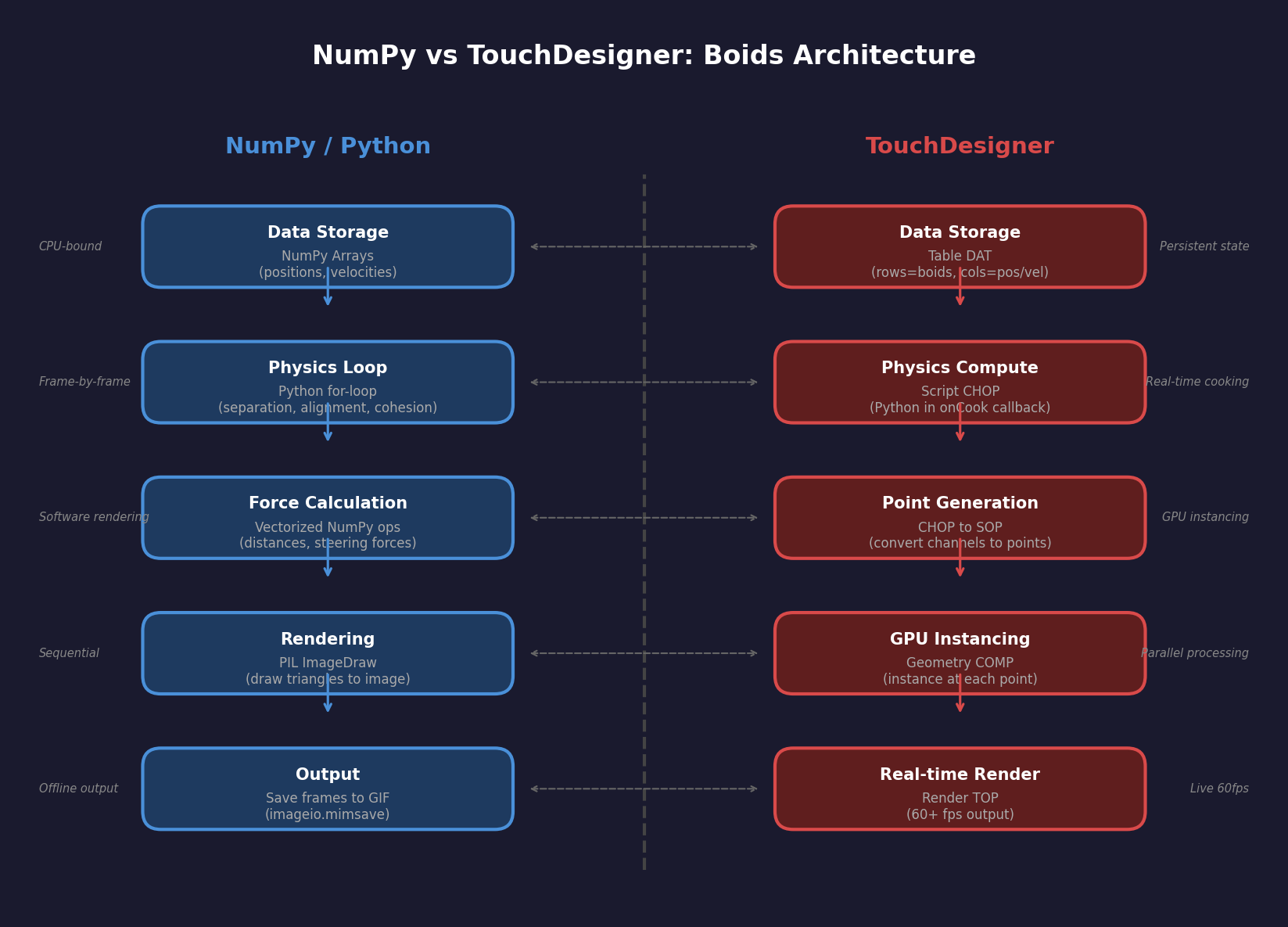
Module 5.2.1 implemented Craig Reynolds’ boids in NumPy. The pure-Python simulation handles 50–100 agents at interactive speed; past that it drops below 30 fps and the visualisation stutters. To run thousands of boids — for a gallery installation, a music-reactive backdrop, or a VR scene — you need to (a) move the physics into a faster execution context and (b) replace per-agent rendering with batched GPU instancing. TouchDesigner is built for both. The physics moves into a Script CHOP that runs once per frame and outputs all agent positions as channel arrays. The rendering moves into a Geometry COMP with GPU instancing — one draw call for any number of agents.

The three boids rules from 5.2.1 — separation, alignment, cohesion — are the same. The data structures are the same (NumPy arrays of positions and velocities). What changes is where the computation lives and how the output is drawn.

Learning objectives

1. Move per-frame physics from a Python script into a Script CHOP whose output is consumed by other operators.
2. Use GPU instancing to render N copies of one geometry from one draw call, replacing N draw calls.
3. Identify the performance crossover point where CPU NumPy is no longer fast enough and GPU/native pipelines become necessary.
4. Recognise the three-tier architecture — physics layer, rendering layer, control layer — that underlies all real-time agent simulations.

Part 1 — Physics in a Script CHOP

A Script CHOP runs a Python onCook callback every frame. It outputs channels — named arrays of float values that other operators can read. For boids, the channels are:

• tx, ty — position (length N)
• vx, vy — velocity (length N)
• (optional) heading — rotation angle for rendering

Inside the script, the per-frame body is essentially the NumPy code from 5.2.1, minus the loop over frames (TD provides that). Read agent state from me.par.X storage, compute separation/alignment/cohesion, update velocity and position, write back to the output channels.

# inside a Script CHOP onCook callback
def onCook(scriptOp):
    n = me.par.Numagents.eval()
    pos = positions      # persisted state (module-level NumPy array)
    vel = velocities

    sep = separation(pos)        # same as 5.2.1
    align = alignment(pos, vel)
    coh = cohesion(pos)
    vel = clip_speed(vel + sep + align + coh, MAX_SPEED)
    pos = (pos + vel) % WORLD_SIZE

    scriptOp.clear()
    scriptOp.appendChan('tx').vals = pos[:, 0].tolist()
    scriptOp.appendChan('ty').vals = pos[:, 1].tolist()
    scriptOp.appendChan('heading').vals = np.degrees(
        np.arctan2(vel[:, 1], vel[:, 0])).tolist()
    return

The state (positions, velocities) is stored as module-level NumPy arrays inside the script. They persist between frames because the script lives in the cook cycle, not in a fresh Python process.

Part 2 — Rendering with GPU instancing

Drawing 5,000 small triangles individually requires 5,000 draw calls. Even at 100 µs per call, that is 500 ms per frame — useless. The cure is GPU instancing: one draw call submits one geometry plus a per-instance attribute array (positions, headings, sizes), and the GPU draws all N copies in parallel.

In TouchDesigner you set this up on the Geometry COMP:

1. Build the agent geometry as a single SOP — a small triangle or sphere.
2. On the Geometry COMP, set Instancing to On.
3. In the Instance page of parameters, point the Translate OP to your physics Script CHOP (the tx, ty channels become per-instance translations).
4. Point the Rotate OP to the same CHOP (the heading channel becomes per-instance rotation).
5. The COMP now draws all N copies in one GPU draw call.

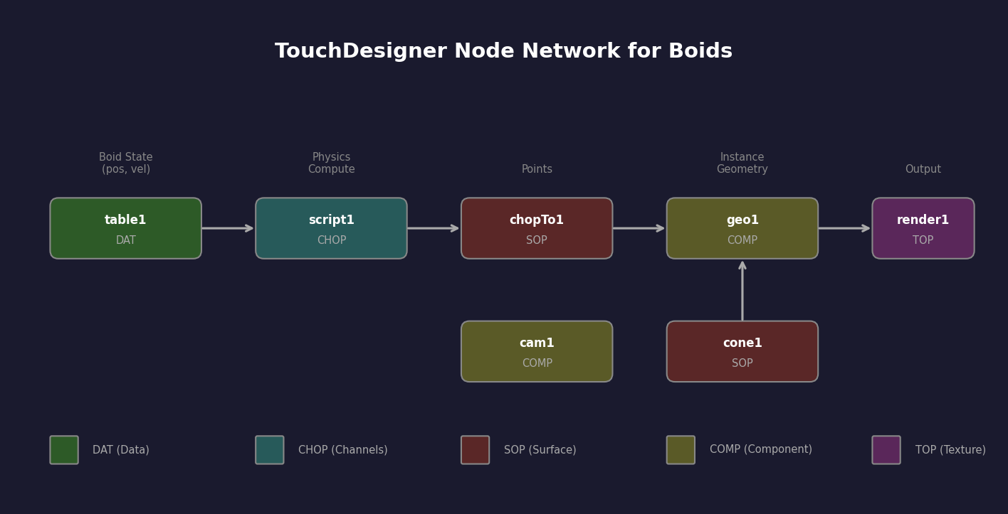
Script CHOP (physics output)
  ╲
   ╲ Translate OP, Rotate OP
    ╲
     Geometry COMP (with instancing on) → Render TOP → Out

Modern GPUs handle 50,000–500,000 instances per frame easily. The bottleneck moves entirely from the rendering side to the physics side — exactly where you can apply NumPy and the GPU-friendly algorithms from Module 7.

Part 3 — Three-tier architecture

The Boids-in-TD setup illustrates a pattern that recurs for every real-time agent simulation:

Physics layer — Script CHOP (or GLSL Compute TOP for very large counts). Inputs: state from previous frame. Outputs: new state as channels.

Rendering layer — Geometry COMP with instancing. Inputs: channels from physics layer. Output: a Render TOP.

Control layer — Script DAT and CHOPs. Inputs: external events (MIDI, OSC, audio). Outputs: parameter changes on the physics layer.

This separation is what lets you scale: optimise the physics layer to run more agents, optimise the rendering layer to draw them faster, and add features in the control layer without touching either. Compare to the NumPy version where adding “respond to audio” means surgery on the inner loop.

Synthesis project — port your 5.2.1 boids to TD

Take the NumPy boids from lesson 5.2.1, drop the physics function into a Script CHOP, wire the output channels to a Geometry COMP with instancing, and watch 500–5,000 boids fly at 60 fps. The .py download is the standalone reference matching the v1 implementation; the .toe project shows the wired TD network.

Reflection questions

• What is the largest single cost in the pure-NumPy 5.2.1 version that disappears in the TD version?
• Why is GPU instancing useless for boids if your geometry is one triangle but heroic if it is a complex sphere mesh?
• At what agent count does pure NumPy stop being competitive with the TD version, and why?

Make it your own

• Audio reactivity: add an Audio In CHOP, compute spectrum, use bass amplitude to modulate cohesion_weight. Boids cluster on drum hits.
• GLSL Compute physics: move the Script CHOP body into a GLSL Compute TOP. Now physics runs on the GPU and you can do 50,000 agents.
• Predator agent: one special agent that all boids flee from; the predator chases the centroid of the flock. Classic stability test for any flocking implementation.

Summary

Common pitfalls to avoid

• Per-agent draw calls instead of instancing. The rendering cost stays O(N) and you cannot scale.
• State stored in script-local variables that disappear each frame. Use module-level globals or me.storage for persistent state.
• Script CHOP reading parameters in Python without .eval(). You get the parameter object, not its value.
• Boids forces computed in a Python loop instead of vectorised NumPy. The O(N²) cost compounds; vectorise like 5.2.1.
• Wiring CHOP channels in wrong order to instancing parameters. Channel order matters; double-check tx, ty, tz and rx, ry, rz mapping.

References

- [1] Reynolds, C. W. (1987). Flocks, herds and schools: A distributed behavioral model. ACM SIGGRAPH Computer Graphics, 21(4), 25–34. doi:10.1145/37402.37406
- [2] Derivative Inc. (2024). TouchDesigner Geometry COMP Documentation. derivative.ca/UserGuide/Geometry_COMP
- [3] Akeley, K., & Hanrahan, P. (1988). Three pieces of the graphics pipeline. Computer Graphics, 22(4), 197–204.
- [4] NVIDIA Corporation. (2022). Instanced Rendering Best Practices. developer.nvidia.com
- [5] Reynolds, C. W. (1999). Steering behaviors for autonomous characters. In Proceedings of Game Developers Conference 1999 (pp. 763–782).
- [6] Shiffman, D. (2012). The Nature of Code, Chapter 6: Autonomous Agents. natureofcode.com