6.1.1 Perlin & Value Noise
Build smooth, organic noise by sampling a random grid and interpolating between cells with a smoothstep. Stack octaves of decreasing amplitude and increasing frequency for cloud-like fractal Brownian motion.
Overview
Random pixel-by-pixel noise looks like television static — every cell independent of its neighbours, no structure at any scale. Ken Perlin’s 1983 insight was that coherent noise (where neighbouring samples are correlated) reads as natural — clouds, smoke, marble veins, terrain [1]. The recipe is two ingredients: a grid of random values, and a smooth interpolation between them. Layer several such noise fields at different scales and you get fractional Brownian motion (fBm), the workhorse of every procedural texture in games and VFX since Tron [2]. This lesson builds the pipeline in NumPy from scratch, so you can read every pixel-level decision.
Learning objectives
- Distinguish random noise (TV static) from coherent noise (Perlin/value noise) — the smoothness comes from interpolating a coarse random grid.
- Implement bilinear interpolation with a smoothstep
S(t) = 3t² − 2t³for the natural-looking transitions. - Combine multiple octaves of noise with halving amplitude (persistence) and doubling frequency (lacunarity) to build fractal Brownian motion.
- Tune
scale,octaves, andpersistenceto move between blobby and detailed textures.
Quick start — value noise clouds
import numpy as np
from PIL import Image

def smoothstep(t):
    return t * t * t * (t * (t * 6 - 15) + 10)        # quintic, Perlin 2002

def value_noise(shape, scale, seed=0):
    h, w = shape
    rng = np.random.default_rng(seed)
    cells_y = int(np.ceil(h / scale)) + 2
    cells_x = int(np.ceil(w / scale)) + 2
    cells = rng.random((cells_y, cells_x))            # random per grid corner

    y, x = np.mgrid[:h, :w].astype(np.float64)
    yf = y / scale; xf = x / scale
    y0 = yf.astype(int); x0 = xf.astype(int)
    ty = smoothstep(yf - y0)
    tx = smoothstep(xf - x0)

    c00 = cells[y0,     x0    ]; c10 = cells[y0 + 1, x0    ]
    c01 = cells[y0,     x0 + 1]; c11 = cells[y0 + 1, x0 + 1]
    top = c00 + (c01 - c00) * tx
    bot = c10 + (c11 - c10) * tx
    return top + (bot - top) * ty                     # in [0, 1]

def fbm(shape, scale, octaves=6, persistence=0.5, seed=0):
    out = np.zeros(shape); amp = 1.0; s = scale; norm = 0
    for o in range(octaves):
        out += amp * value_noise(shape, s, seed + o)
        norm += amp; amp *= persistence; s /= 2
    return out / norm

z = fbm((512, 512), scale=90, octaves=6, seed=7)
img = (z * 255).astype(np.uint8)
Image.fromarray(img, 'L').save('value_clouds.png')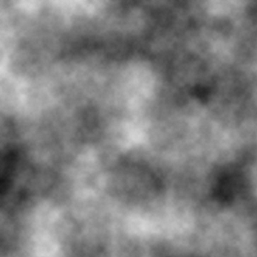
Core concepts
Concept 1 — Random vs coherent
Pure random per-pixel noise produces TV-static — every neighbour is independent:
rng = np.random.default_rng(7)
static = rng.random((256, 256))     # white noise
Coherent noise samples a coarse random grid (say one cell per 30 pixels), then interpolates between the corners. Adjacent pixels in the output share most of their nearby grid values, so they take on similar interpolated values — neighbours look alike.
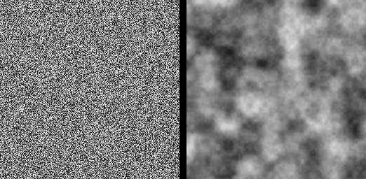
Concept 2 — Smoothstep interpolation
A naive linear interpolation between corner values gives visible diamond patterns at cell boundaries because the derivative changes abruptly at each crossing. Ken Perlin’s 2002 fix replaced the cubic smoothstep 3t² − 2t³ with a quintic 6t⁵ − 15t⁴ + 10t³ whose first and second derivatives both vanish at t = 0 and t = 1 [1].
def smoothstep(t):
    return t * t * t * (t * (t * 6 - 15) + 10)
t = 0→0,S′(0) = 0,S″(0) = 0.t = 1→1,S′(1) = 0,S″(1) = 0.
The result is invisible cell boundaries even under derivative-amplifying operations like edge detection.
Concept 3 — Fractional Brownian motion (fBm)
A single octave of noise is too smooth — it has features at exactly one scale. Adding multiple octaves at halving amplitude and doubling frequency layers detail without overwhelming the base shape. The result is fractional Brownian motion, the same mathematical object that describes Brownian particle paths and natural terrain [4]:
total = octave_1 + (1/2) * octave_2 + (1/4) * octave_3 + (1/8) * octave_4 + ...Each subsequent octave halves the wavelength (lacunarity = 2) and halves the amplitude (persistence = 0.5).
Exercises
Three exercises in Execute → Modify → Create order: run the cloud generator, tune octaves and persistence, then build a blue-tinted cloud panorama.
Run the cloud generator
Run value_clouds.py from the downloads. Inspect the output.
Reflection questions
- Why does
fbmdivide bynormat the end? - What happens if you drop
octavesto1? - What happens if you raise
persistenceto0.9?
Answers
/ norm — without it, the sum of octaves overshoots the unit range. norm accumulates the same geometric series as amp, so dividing rescales the result back into [0, 1] regardless of how many octaves you stacked.
1 octave — the picture becomes a soft blobby field with features at exactly the base scale (90 pixels here). No fine detail; reads as a depth gradient rather than a texture.
Persistence 0.9 — higher octaves contribute almost as much as the base. The texture turns coarse and rough; the larger-scale features get drowned in the high-frequency content. Useful when you want noise; less useful when you want clouds.
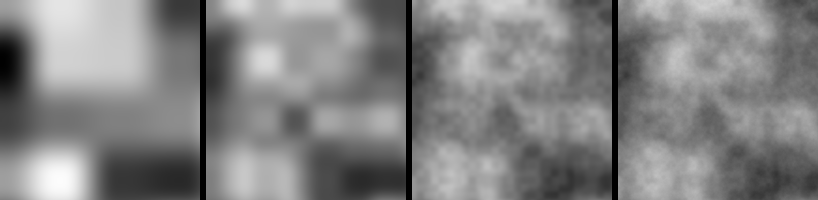
Three parameter sweeps
Edit value_clouds.py to produce these three pictures.
Goals
- Big features — bump
scaleto200and watch the texture zoom out. - Fewer layers — drop
octavesto2for blobby contour-like output. - Smoother decay — set
persistence=0.3to suppress fine detail.
Goal 1 — what to expect
z = fbm((512, 512), scale=200, octaves=6, seed=7)Each cell is now 200 pixels. You see only a handful of large rolling shapes instead of many small ones.
Goal 2 — what to expect
z = fbm((512, 512), scale=90, octaves=2, seed=7)Two octaves: a base shape with one layer of medium detail. The texture reads as topography rather than clouds.
Goal 3 — what to expect
z = fbm((512, 512), scale=90, octaves=6, persistence=0.3, seed=7)Fine octaves contribute much less. The picture stays soft even at six octaves — useful for distant fog or smooth depth fields.
Blue-tinted clouds over a colour gradient
Render the noise as a soft blue cloud field by stuffing the noise value into the red and green channels and keeping blue near 1. Then add a vertical sky gradient under the clouds.
import numpy as np
from PIL import Image
# ... assume fbm() from quick start is defined ...

H, W = 320, 640
z = fbm((H, W), scale=110, octaves=5, seed=42)

# TODO 1: build a sky gradient — RGB that goes from a deep blue at top
#         to a paler blue at the horizon.

# TODO 2: build a cloud overlay: white where z is high, transparent where low.
#         Multiply-screen the cloud onto the sky.

Image.fromarray(rgb_uint8).save('blue_clouds.png')
Hint 1 — sky gradient
sky_top = np.array([0.30, 0.50, 0.85])
sky_bot = np.array([0.80, 0.90, 1.00])
yy = np.linspace(0, 1, H)[:, None, None]
sky = sky_top * (1 - yy) + sky_bot * yy
sky = np.broadcast_to(sky, (H, W, 3)).copy()
Hint 2 — cloud overlay
cloud = np.clip((z - 0.45) * 4, 0, 1)             # threshold + amplify
out = sky * (1 - cloud[..., None]) + cloud[..., None] * 1.0
rgb_uint8 = (np.clip(out, 0, 1) * 255).astype(np.uint8)
Complete solution
import numpy as np
from PIL import Image

def smoothstep(t):
    return t * t * t * (t * (t * 6 - 15) + 10)

def value_noise(shape, scale, seed=0):
    h, w = shape
    rng = np.random.default_rng(seed)
    cells = rng.random((int(np.ceil(h/scale)) + 2, int(np.ceil(w/scale)) + 2))
    y, x = np.mgrid[:h, :w].astype(float)
    yf = y/scale; xf = x/scale
    y0 = yf.astype(int); x0 = xf.astype(int)
    ty = smoothstep(yf - y0); tx = smoothstep(xf - x0)
    c00 = cells[y0, x0];     c10 = cells[y0+1, x0]
    c01 = cells[y0, x0+1];   c11 = cells[y0+1, x0+1]
    top = c00 + (c01 - c00) * tx; bot = c10 + (c11 - c10) * tx
    return top + (bot - top) * ty

def fbm(shape, scale, octaves=5, persistence=0.5, seed=0):
    out = 0; amp = 1.0; s = scale; norm = 0
    for o in range(octaves):
        out = out + amp * value_noise(shape, s, seed + o)
        norm += amp; amp *= persistence; s /= 2
    return out / norm

H, W = 320, 640
z = fbm((H, W), scale=110, octaves=5, seed=42)

sky_top = np.array([0.30, 0.50, 0.85])
sky_bot = np.array([0.80, 0.90, 1.00])
yy = np.linspace(0, 1, H)[:, None, None]
sky = sky_top * (1 - yy) + sky_bot * yy
sky = np.broadcast_to(sky, (H, W, 3)).copy()

cloud = np.clip((z - 0.45) * 4, 0, 1)
out = sky * (1 - cloud[..., None]) + cloud[..., None] * 1.0
rgb = (np.clip(out, 0, 1) * 255).astype(np.uint8)
Image.fromarray(rgb).save('blue_clouds.png')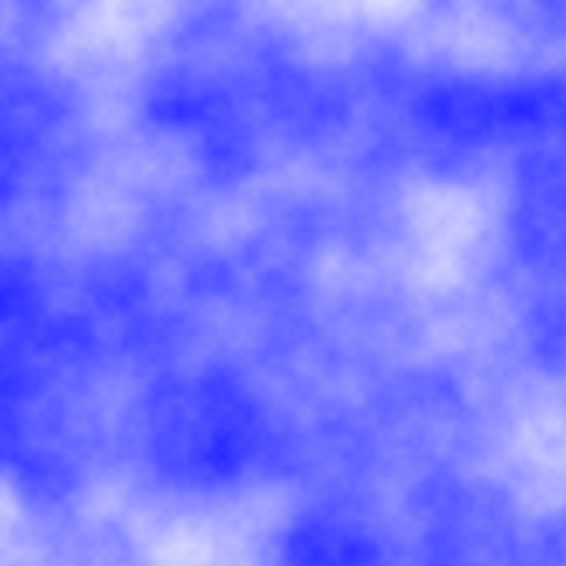
How it works:
- The sky gradient is a vertical lerp from a saturated blue to a pale blue.
cloud = clip((z - 0.45) * 4, 0, 1)thresholds and amplifies — values below 0.45 are zero (no cloud), values above quickly saturate to white.- The final composite uses the cloud mask as alpha: cloudy regions go white, clear regions show the gradient sky.
Make it your own
- Switch the colour ramp to evening — saturated orange at the horizon, deep purple at the zenith. The same noise reads as sunset clouds.
- Swap value noise for the gradient version (Perlin). Implement it by storing 2D unit vectors at each grid corner and replacing
cells[...]reads with dot products against(yf − y0, xf − x0). - Animate
seedfrom 0 to 60 and assemble a GIF — the clouds drift coherently because each frame is one step along an underlying noise lattice.
Downloads
value_clouds.png — quick-start output reference octaves_grid.png — octave comparison perlin_clouds.png — v1 cloud reference (noise library)Summary
Common pitfalls to avoid
- Linear interpolation instead of smoothstep — visible cell grid in the output.
- Using
np.random.randomper pixel — that is white noise, not value noise; the smoothness comes from interpolating a coarse grid. - Forgetting to normalise after summing octaves — the value range drifts above 1, and
(z * 255).astype(uint8)saturates. - Persistence above 1 — higher octaves dominate the lower ones; the texture turns into noise.
- Reusing the same seed across octaves — same noise patterns at different scales line up suspiciously. Offset the seed by the octave index.
References
- [1] Perlin, K. (1985). An image synthesizer. ACM SIGGRAPH Computer Graphics, 19(3), 287–296. doi:10.1145/325165.325247
- [2] Perlin, K. (2002). Improving noise. ACM Transactions on Graphics, 21(3), 681–682. doi:10.1145/566654.566636
- [3] Ebert, D. S., Musgrave, F. K., Peachey, D., Perlin, K., & Worley, S. (2003). Texturing and Modeling: A Procedural Approach (3rd ed.). Morgan Kaufmann.
- [4] Mandelbrot, B. B., & Van Ness, J. W. (1968). Fractional Brownian motions, fractional noises and applications. SIAM Review, 10(4), 422–437. doi:10.1137/1010093
- [5] Lagae, A., Lefebvre, S., Cook, R., et al. (2010). A survey of procedural noise functions. Computer Graphics Forum, 29(8), 2579–2600. doi:10.1111/j.1467-8659.2010.01827.x
- [6] Harris, C. R., Millman, K. J., van der Walt, S. J., et al. (2020). Array programming with NumPy. Nature, 585, 357–362. doi:10.1038/s41586-020-2649-2