5.1.1 Sand Simulation
Build a particle system from scratch — thousands of independent grains, each carrying a few floats of state, animated frame by frame into a GIF of wind-blown sand.
Overview
Watch sand blow across a desert and what looks like one shifting carpet is actually thousands of grains, each moving on its own. A particle system is the computational mirror of that observation: many small agents, each with a tiny piece of state — position, velocity, colour — updated under the same simple rules every frame. William Reeves invented this technique at Lucasfilm in 1982 for the Genesis sequence in Star Trek II, and the same pattern now powers smoke in games, sparks in films, and the digital sand you will build here [1]. By the end of this lesson you will have a GIF of roughly 6,700 grains drifting and accelerating to the right, generated from one Python script and one tight render loop.
Learning objectives
- Model a particle as an object with float-valued position, velocity, and per-particle delay, colour, and state.
- Apply Euler integration —
position += velocity,velocity *= acceleration— to thousands of agents per frame. - Use a Gaussian distribution to stagger particle start times so the flock peels away naturally rather than marching in lockstep.
- Render each frame into a NumPy array and assemble the sequence into an animated GIF with
imageio.
Quick start — watch the sand blow away
The minimum viable particle system: 500 grains, eighty frames, exactly one acceleration rule.
import random
import numpy as np
from PIL import Image
import imageio.v2 as imageio
particles = []
for _ in range(500):
particles.append({
'x': 150 + random.randint(0, 100),
'y': 100 + random.randint(0, 100),
'vx': random.uniform(-1, 2),
'vy': random.uniform(-0.5, 0.5),
'delay': random.randint(0, 60),
})
frames = []
for frame in range(80):
img = np.zeros((200, 300, 3), dtype=np.uint8)
for p in particles:
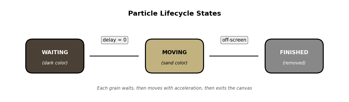
if p['delay'] > 0:
p['delay'] -= 1
colour = (50, 40, 30)
else:
p['x'] += p['vx']
p['y'] += p['vy']
p['vx'] *= 1.05
colour = (194, 178, 128)
x, y = int(p['x']), int(p['y'])
if 0 <= x < 297 and 0 <= y < 197:
img[y:y + 3, x:x + 3] = colour
frames.append(img)
imageio.mimsave('quick_sand.gif', frames, fps=24)
Core concepts
Concept 1 — A particle is a bag of state
A particle system is a collection of small independent objects, each carrying its own state. Every particle in our sand simulation owns:
- a position
(x, y)in canvas pixels (stored as floats, so motion can be sub-pixel), - a velocity
(vx, vy)in pixels per frame, - a delay counting down to when this grain starts moving,
- a colour sampled with small per-grain jitter so the dune does not look painted.
The state lives on the particle itself — there is no shared global update — which is what makes particle systems trivially parallelisable on a GPU and easy to extend. Add a radius field and you can simulate raindrops of varying sizes. Add an age field and you can fade particles over time. The architecture is open by default.
Concept 2 — Euler integration in two lines
Particles move by the cheapest possible numerical-integration rule: Euler’s method. New position equals old position plus velocity; new velocity equals old velocity times an acceleration multiplier.
def update(self):
    self.x += self.velocity_x
    self.y += self.velocity_y

    if self.velocity_x < 1.0:
        self.velocity_x += 0.2     # nudge leftward-moving grains rightward
    else:
        self.velocity_x *= 1.08    # exponential speed-up once moving right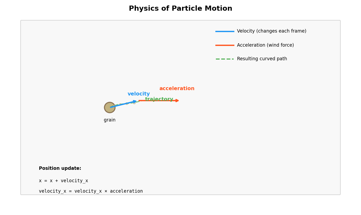
Euler is not the most accurate integrator — it accumulates error over long simulations, which is why we will switch to RK4 in lesson 5.3.3 — but for short animations of small, fast-moving objects it is perfect. The reason floats matter here is sub-pixel motion: self.x += 0.3 does nothing visible by itself, but after ten frames the grain has moved three pixels. Integer positions would round those increments to zero and the simulation would freeze.
Concept 3 — Gaussian delays for natural variation
If every grain starts at frame zero, the wind looks like a shove. If they start at evenly-spaced intervals, it looks mechanical. Real sand has clustered variation — most grains move around the same time, with a few stragglers and a few that jump early. That is a Gaussian distribution.
import random

self.delay = max(0, int(random.gauss(50, 15)))
random.gauss(50, 15) draws a sample centred at frame 50 with a standard deviation of 15 — so roughly two-thirds of grains start between frames 35 and 65, with a small minority outside that band. The max(0, ...) clamps the rare negative draws so no grain has a “negative delay”.
Exercises
Three exercises in Execute → Modify → Create order: run the desert as it ships, retune four parameters, then build your own particle effect on top of the same engine.
Run the desert
Download sand_simulation.py and run it. It will print progress and write sand_animation.gif to the current folder.
Reflection questions
- Why do the grains not all start moving at the same time? What visual effect does that create?
- Follow one grain with your eyes. Does it travel in a straight line, or does it curve?
- Watch grains far to the right. Are they speeding up, slowing down, or moving at constant speed?
Answers
Staggered starts — each grain draws its delay from random.gauss(50, 15). The Gaussian peaks at frame 50 but spreads across roughly frames 20–80, so the desert peels away in waves rather than as one moving block. That peel mirrors how real wind lifts loose particles unevenly.
Curved paths — the initial velocity_y is small but nonzero, so each grain drifts vertically as well as horizontally. That tiny perpendicular component is what makes the trajectory look “turbulent” instead of ruler-straight.
Exponential speed-up — once a grain’s velocity_x exceeds 1, the update applies velocity_x *= 1.08, which is geometric growth. After thirty moving frames a grain is ten times faster than when it started. That is the visual signature of acceleration as opposed to drift.
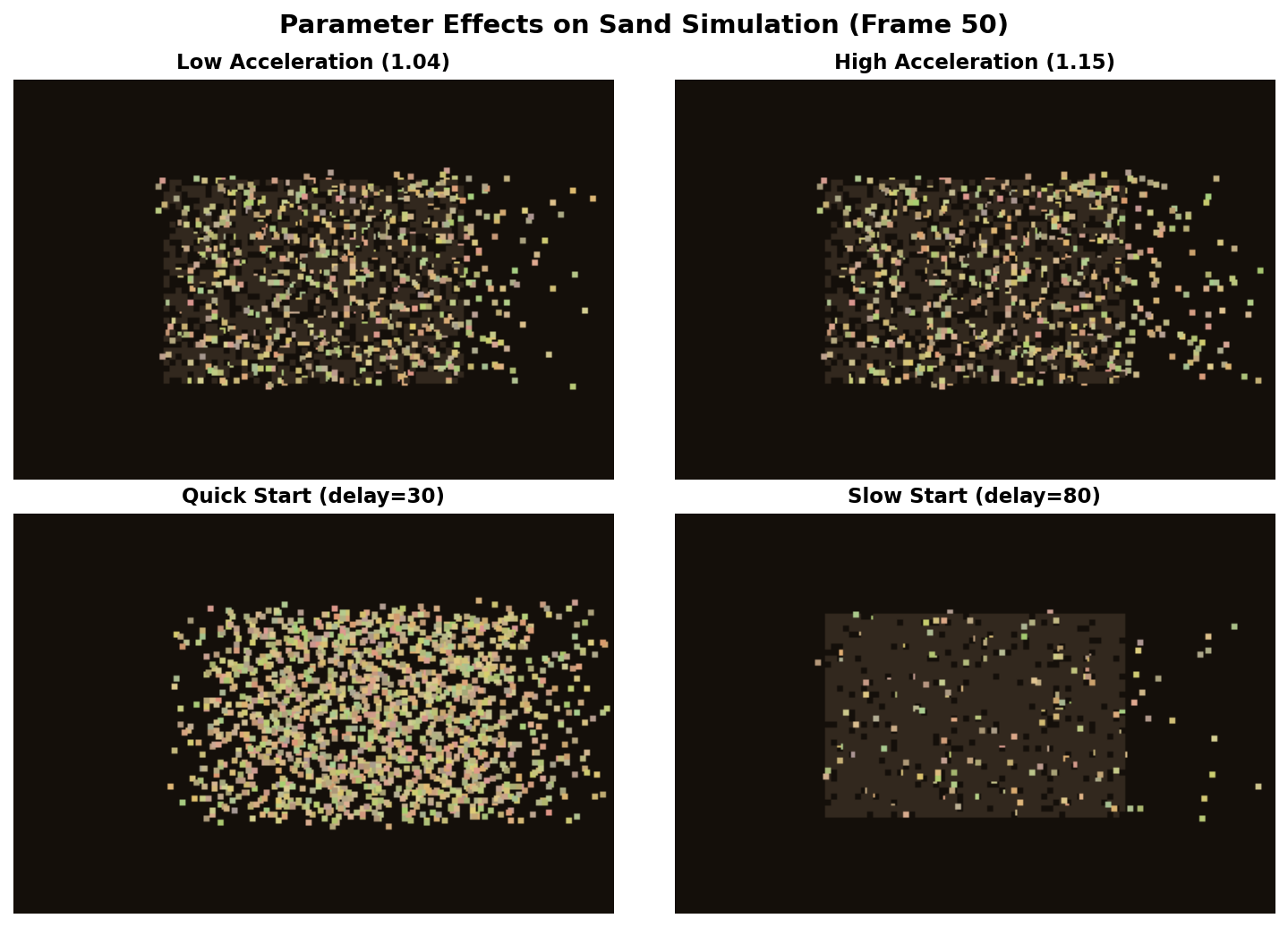
Retune the wind
Open your copy of sand_simulation.py and change one variable at a time. Re-render the GIF and confirm each modification produces the expected effect.
Goals
- Reverse the wind: make sand blow left instead of right.
- Add gravity: make sand fall straight down like an hourglass.
- Fast start: collapse the Gaussian delay to frames 0–20 so the whole desert moves at once.
- Sunset palette: swap the beige base for orange/red so the sand looks like Mars.
Goal 1 — what to expect
In update, flip the sign of the acceleration:
if self.velocity_x > -1.0:
    self.velocity_x -= 0.2
else:
    self.velocity_x *= 1.08
Also flip the exit check (self.x <= 0) so off-canvas-left grains finish. The desert reads right-to-left and the dark “waiting” pixels are revealed in reverse.
Goal 2 — what to expect
Accelerate velocity_y instead of velocity_x. A constant downward +0.3 per frame mimics gravity (sand on Earth falls at 9.81 m/s², but we are working in pixels per frame so this is a unit choice rather than a physics fact). The grains stream straight down, fanning slightly because each one starts at a different x.
Goal 3 — what to expect
self.delay = max(0, int(random.gauss(10, 5))). Now most delays fall in the 5–15 range. The whole field starts moving by frame 20, which trades the “peeling” effect for a uniform shove. Useful when you want a single gust rather than a continuous wind.
Goal 4 — what to expect
Set SAND_BASE = (255, 120, 50) and shift the per-grain colour jitter toward reds and yellows:
self.color = (
    random.randint(200, 255),
    random.randint(50, 150),
    random.randint(0, 50),
)
The desert now reads as Mars — same physics, different palette. Colour is the cheapest narrative tool in generative art.
Build your own particle effect
Use sand_simulation_starter.py as a base and implement one of these three effects from scratch. The engine — the per-frame loop, the rendering, the GIF save — stays the same; you change the Particle class and the spawning logic.
Choose one
- Rain drops — spawn at the top edge, fall straight down with slight horizontal drift, vanish at the bottom.
- Rising bubbles — spawn at the bottom edge, float upward, add a small sine wiggle to the x-position so they look effervescent.
- Confetti burst — spawn all particles at the centre, give each one a random direction-of-explosion, apply friction so they decelerate naturally.
Rain drops — solution sketch
class Particle:
    def __init__(self, x, y):
        self.x, self.y = float(x), float(y)
        self.is_active = True
        self.velocity_x = random.uniform(-0.3, 0.3)
        self.velocity_y = random.uniform(3, 5)
        self.color = (
            random.randint(150, 200),
            random.randint(200, 230),
            255,
        )

    def update(self):
        if not self.is_active:
            return
        self.x += self.velocity_x
        self.y += self.velocity_y
        if self.y > HEIGHT:
            self.is_active = False
Spawn along the full width at y = random.randint(-50, 0) so drops trickle in rather than appearing all at once.
Rising bubbles — solution sketch
import math

class Particle:
    def __init__(self, x, y):
        self.x, self.y = float(x), float(y)
        self.is_active = True
        self.velocity_y = random.uniform(-2, -1)
        self.phase = random.uniform(0, 2 * math.pi)
        self.age = 0
        self.color = (
            random.randint(100, 150),
            random.randint(200, 230),
            255,
        )

    def update(self):
        if not self.is_active:
            return
        self.age += 1
        self.x += math.sin(self.age * 0.1 + self.phase) * 0.5
        self.y += self.velocity_y
        if self.y < 0:
            self.is_active = False
Each bubble has its own phase so the wiggle is desynchronised — without that, every bubble would weave left and right in lockstep and the swarm would look like a marching band.
Confetti burst — solution sketch
import math

class Particle:
    def __init__(self, x, y):
        self.x, self.y = float(x), float(y)
        self.is_active = True
        angle = random.uniform(0, 2 * math.pi)
        speed = random.uniform(3, 8)
        self.velocity_x = math.cos(angle) * speed
        self.velocity_y = math.sin(angle) * speed
        self.color = (
            random.randint(100, 255),
            random.randint(100, 255),
            random.randint(100, 255),
        )

    def update(self):
        if not self.is_active:
            return
        self.x += self.velocity_x
        self.y += self.velocity_y
        self.velocity_x *= 0.98  # friction
        self.velocity_y *= 0.98
        self.velocity_y += 0.1   # gravity
        if self.x < 0 or self.x > WIDTH or self.y > HEIGHT:
            self.is_active = False
Spawning all particles at the centre with uniformly-random angles produces a clean circular burst. Adding the small gravity term makes it sag — the difference between fireworks and a soap-bubble pop.
Make it your own
- Stack two systems: a “rocket” rises, then at its apex spawns 50 confetti particles. That is a one-shot firework.
- Replace the
delaycountdown with a per-particlelifetimeso grains fade after they have travelled a fixed number of frames. Now the desert breathes. - Render onto a slowly-darkening background so trails persist for a few frames. Cheap motion-blur for free.
Downloads
sand.py — minimal quick-start used in the Overview sand_simulation.py — full reference implementation sand_simulation_starter.py — Exercise 3 scaffoldSummary
Common pitfalls to avoid
- Storing
xandyas ints. Sub-pixel motion vanishes and the grains freeze. - Forgetting the off-canvas check. Particles that fly away forever still cost compute every frame.
- Same delay for every grain. The desert lurches as one block; the eye reads it as one rigid object.
- Skipping the
max(0, ...)clamp onrandom.gauss. A negative delay means a grain that started “in the past” — usually harmless, occasionally a crash. - Spawning ten thousand particles before the loop is fast. Profile on a hundred first.
References
- [1] Reeves, W. T. (1983). Particle systems: A technique for modeling a class of fuzzy objects. ACM SIGGRAPH Computer Graphics, 17(3), 359–375. doi:10.1145/964967.801167
- [2] Shiffman, D. (2012). The Nature of Code, Chapter 4: Particle Systems. natureofcode.com
- [3] Sims, K. (1990). Particle animation and rendering using data parallel computation. ACM SIGGRAPH Computer Graphics, 24(4), 405–413.
- [4] Reynolds, C. W. (1987). Flocks, herds and schools: A distributed behavioral model. ACM SIGGRAPH Computer Graphics, 21(4), 25–34. doi:10.1145/37402.37406
- [5] Harris, C. R., et al. (2020). Array programming with NumPy. Nature, 585, 357–362. doi:10.1038/s41586-020-2649-2
- [6] Burden, R. L., & Faires, J. D. (2015). Numerical Analysis (10th ed.), Chapter 5: Initial-Value Problems for Ordinary Differential Equations. Cengage Learning.
- [7] Klein, A., et al. (2024). imageio: Python library for reading and writing image data. imageio.readthedocs.io