2.1.1 Drawing Lines

Overview

A mathematical line is a continuous object — infinitely many points between two endpoints. A computer screen is a discrete grid of pixels with integer coordinates. The whole field of rasterization exists to bridge that gap, and the line is its simplest case. In this lesson you will draw lines by interpolation, then turn the same three-line draw_line function into a sunburst by varying its endpoints inside a loop. The conceptual thread — iteration plus simple rules equals emergent pattern — runs through every later lesson in this module [1].

Learning objectives

1. Understand the rasterization problem: converting continuous line equations into discrete pixel coordinates.
2. Implement parametric line interpolation using NumPy’s linspace, with proper rounding before integer cast.
3. Recognise lines as a generative primitive — iteration over endpoints produces sunbursts, parallel bands, and radial compositions.
4. Connect the algorithmic approach to the conceptual tradition of LeWitt and Molnár, where the instruction is the artwork.

Quick start — one diagonal line

import numpy as np
from PIL import Image

canvas = np.zeros((400, 400), dtype=np.uint8)

# Endpoints in (x, y) pixel coordinates
x_start, y_start = 50, 50
x_end, y_end = 350, 350

# Generate enough sample points to fill every pixel along the longer axis
num_points = max(abs(x_end - x_start), abs(y_end - y_start)) + 1

x_coords = np.linspace(x_start, x_end, num_points).round().astype(int)
y_coords = np.linspace(y_start, y_end, num_points).round().astype(int)

# Array indexing is [row, column] = [y, x]
canvas[y_coords, x_coords] = 255

Image.fromarray(canvas).save('simple_line.png')

Core concepts

Concept 1 — Rasterizing a continuous line

In maths a line is the set of points satisfying $y = mx + b$, or in parametric form $(x(t), y(t))$ with $t \in [0, 1]$. Both descriptions are continuous: between any two points on the line, there are infinitely many more [2]. A screen does not work that way. It is a grid of integer-indexed cells, and a single pixel either belongs to the line or it does not.

The conversion problem — picking which discrete pixels best represent a continuous line — has a long history. Jack Bresenham’s 1965 algorithm solved it with only integer addition and bit shifts, which mattered enormously for the IBM 2250 pen plotters of the era, since those plotters had no floating-point hardware at all [3]. Modern Python does not have that constraint, so we lean on np.linspace and let NumPy handle the arithmetic.

Concept 2 — linspace as a parametric interpolator

The parametric line is the cleaner mental model:

$$P(t) = (1 - t),P_0 + t,P_1, \quad t \in [0, 1]$$

At $t = 0$ you are at the start, at $t = 1$ you are at the end, and at $t = 0.5$ you are at the midpoint. This blending operation — linear interpolation, often shortened to “lerp” — underlies most of computer graphics: animation keyframes, colour gradients, image scaling, Bézier curves [4].

NumPy’s linspace is this interpolation, applied to a single axis:

import numpy as np

# 5 evenly-spaced points from 0 to 10
points = np.linspace(0, 10, 5)
# → array([ 0. ,  2.5,  5. ,  7.5, 10. ])

# Run it on both axes to interpolate a 2D line
x_coords = np.linspace(50, 350, 301)
y_coords = np.linspace(50, 350, 301)

The output is floating-point. Pixel indices must be integers, so we round and cast: .round().astype(int). Skipping the round() is a classic source of dotted lines — astype(int) truncates rather than rounds, so 2.9 becomes 2, and a diagonal can drop pixels along the way.

Concept 3 — Lines as generative primitives

Once draw_line exists, generative art is a question of where you put the endpoints. The earliest computer artists understood this immediately. Vera Molnár wrote programs that systematically varied parameters of geometric compositions in the 1960s [5]. Sol LeWitt, working without computers, wrote instructions — “wall drawings” — that other people executed, treating the instruction set itself as the artwork [6]. Both were doing what we do here: defining a rule, then iterating it.

# A sunburst: 24 lines from a centre point to evenly-spaced angles
import numpy as np
from PIL import Image

canvas = np.zeros((400, 400), dtype=np.uint8)
cx, cy, radius = 200, 200, 180

angles = np.linspace(0, 2 * np.pi, 24, endpoint=False)
for theta in angles:
    ex = int(cx + radius * np.cos(theta))
    ey = int(cy + radius * np.sin(theta))
    n = max(abs(ex - cx), abs(ey - cy)) + 1
    xs = np.linspace(cx, ex, n).round().astype(int)
    ys = np.linspace(cy, ey, n).round().astype(int)
    canvas[ys, xs] = 255

Image.fromarray(canvas).save('sunburst.png')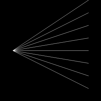

The endpoint (int(cx + radius * cos(theta)), int(cy + radius * sin(theta))) is the polar-to-Cartesian conversion. Multiplying the unit circle by radius scales it, adding (cx, cy) translates it. You are not drawing a circle — you are drawing 24 straight lines whose endpoints happen to land on a circle.

Exercises

Three exercises in Execute → Modify → Create order: run a working line script, vary its parameters, then build a sunburst from scratch.

import numpy as np
from PIL import Image

canvas = np.zeros((400, 400), dtype=np.uint8)

x_start, y_start = 50, 50
x_end, y_end = 350, 350

num_points = max(abs(x_end - x_start), abs(y_end - y_start)) + 1

x_coords = np.linspace(x_start, x_end, num_points).round().astype(int)
y_coords = np.linspace(y_start, y_end, num_points).round().astype(int)

canvas[y_coords, x_coords] = 255

Image.fromarray(canvas).save('simple_line.png')

x_start, y_start = 50, 200
x_end, y_end = 350, 200

x_start, y_start = 200, 50
x_end, y_end = 200, 350

canvas = np.zeros((400, 400), dtype=np.uint8)

for i in range(5):
    offset = i * 40
    x_start, y_start = 50, 50 + offset
    x_end, y_end = 350, 350 + offset

    num_points = max(abs(x_end - x_start), abs(y_end - y_start)) + 1
    x_coords = np.linspace(x_start, x_end, num_points).round().astype(int)
    y_coords = np.linspace(y_start, y_end, num_points).round().astype(int)

    canvas[y_coords, x_coords] = 255

Image.fromarray(canvas).save('parallel.png')

CREATE III.

Sunburst with at least 16 rays

Build a sunburst: lines radiating from the centre of the canvas to evenly-spaced points on a circle around it.

Goal: at least 16 rays from (200, 200) to points on a circle of radius 180, on a 400×400 canvas.

Approach

• Use np.linspace(0, 2 * np.pi, num_rays, endpoint=False) to get the angles. endpoint=False prevents the first and last angle from landing on the same pixel.
• For each angle, compute the ray endpoint with (cx + r*cos(theta), cy + r*sin(theta)).
• Reuse your draw_line logic — wrap it in a function if you have not already.

python · exercise3_starter.py Copy

import numpy as np
from PIL import Image

def draw_line(canvas, x0, y0, x1, y1):
    # TODO 1: copy the linspace-based line drawing into this function
    pass

canvas = np.zeros((400, 400), dtype=np.uint8)
cx, cy = 200, 200
radius = 180
num_rays = 24

# TODO 2: generate num_rays evenly-spaced angles from 0 to 2*pi
# angles = ...

# TODO 3: for each angle, compute the endpoint (ex, ey) and call draw_line
# for theta in angles:
#     ex = ...
#     ey = ...
#     draw_line(canvas, cx, cy, ex, ey)

Image.fromarray(canvas).save('sunburst.png')

Hint 1 — generalise `draw_line`

Move the linspace/round/astype(int)/index-assignment block from earlier exercises into a function:

python Copy

def draw_line(canvas, x0, y0, x1, y1):
    n = max(abs(x1 - x0), abs(y1 - y0)) + 1
    xs = np.linspace(x0, x1, n).round().astype(int)
    ys = np.linspace(y0, y1, n).round().astype(int)
    canvas[ys, xs] = 255

Hint 2 — generate angles

angles = np.linspace(0, 2 * np.pi, num_rays, endpoint=False)

This produces 24 angles starting at 0 and ending just before 2*pi. Setting endpoint=False keeps 0 and 2*pi from collapsing onto the same ray.

Hint 3 — polar to Cartesian

For each angle, the ray endpoint is offset from the centre by radius units in the direction of the angle:

ex = int(cx + radius * np.cos(theta))
ey = int(cy + radius * np.sin(theta))

cos and sin together trace out a unit circle. Multiplying by radius scales it; adding (cx, cy) shifts the centre.

Complete solution

python · exercise3_solution.py Copy

import numpy as np
from PIL import Image

def draw_line(canvas, x0, y0, x1, y1):
    n = max(abs(x1 - x0), abs(y1 - y0)) + 1
    xs = np.linspace(x0, x1, n).round().astype(int)
    ys = np.linspace(y0, y1, n).round().astype(int)
    canvas[ys, xs] = 255

canvas = np.zeros((400, 400), dtype=np.uint8)
cx, cy = 200, 200
radius = 180
num_rays = 24

angles = np.linspace(0, 2 * np.pi, num_rays, endpoint=False)
for theta in angles:
    ex = int(cx + radius * np.cos(theta))
    ey = int(cy + radius * np.sin(theta))
    draw_line(canvas, cx, cy, ex, ey)

Image.fromarray(canvas).save('sunburst.png')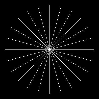

How it works:

• np.linspace(0, 2*np.pi, 24, endpoint=False) gives 24 angles, none of them duplicates.
• The polar-to-Cartesian conversion converts each angle into a Cartesian pixel coordinate on the circle.
• draw_line does the same linspace trick from the quick start — once for each ray. The “circle” never appears in code; it is implied by where the rays terminate.

Make it your own

• Alternate between two radii (radius = 90 on odd rays, 180 on even) for a sharper, star-like silhouette.
• Add a hue by rendering on an RGB canvas — multiply each ray’s intensity by i / num_rays for a colour gradient.
• Increase num_rays to 360 and the sunburst tightens into something close to a filled disc — note how rasterization aliases the rays as they converge.

Downloads

Summary

Common pitfalls to avoid

• Truncating instead of rounding — .astype(int) alone drops fractional parts, leaving dotted lines.
• Swapping (x, y) and (row, col) — NumPy indexes as canvas[row, col], i.e. canvas[y, x]. The y-axis comes first.
• Too few sample points — picking min instead of max for num_points undersamples the longer axis.
• Forgetting endpoint=False on angle arrays — the first and last ray collide on the same pixels.
• Using np.random.rand() (floats in 0–1) as image data — Pillow wants uint8 in 0–255.

References

- [1] Galanter, P. (2003). What is generative art? Complexity theory as a context for art theory. In Proceedings of the 6th Generative Art Conference. Politecnico di Milano.
- [2] Foley, J. D., van Dam, A., Feiner, S. K., & Hughes, J. F. (1990). Computer Graphics: Principles and Practice (2nd ed.). Addison-Wesley.
- [3] Bresenham, J. E. (1965). Algorithm for computer control of a digital plotter. IBM Systems Journal, 4(1), 25–30. doi:10.1147/sj.41.0025
- [4] Gonzalez, R. C., & Woods, R. E. (2018). Digital Image Processing (4th ed.). Pearson.
- [5] Molnár, V. (1974). Toward aesthetic guidelines for paintings with the aid of a computer. Leonardo, 7(3), 185–189. doi:10.2307/1572906
- [6] LeWitt, S. (1967). Paragraphs on conceptual art. Artforum, 5(10), 79–83.
- [7] NumPy Community. (2024). numpy.linspace. NumPy Documentation. numpy.org