9.1.2 Backpropagation Visualisation

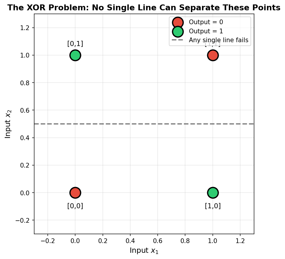
Big question

How does a neural network with hidden layers learn? A single perceptron can’t solve XOR — there is no straight line that separates the points. Adding a hidden layer of perceptrons gives the network enough flexibility to learn a curved boundary, but presented a new problem: how do you adjust the hidden weights when you can only observe the output error? The answer is backpropagation, the chain-rule trick rediscovered for neural networks by Rumelhart, Hinton, and Williams in 1986 [1]. This lesson trains a 2-2-1 network on XOR and traces each gradient step so the math feels concrete.

Learning objectives

1. Build a tiny network with two inputs, two hidden neurons, and one output — about 9 parameters total.
2. Run the forward pass to compute hidden activations and output prediction.
3. Run the backward pass to compute gradients via the chain rule.
4. Apply gradient descent updates to all weights and watch the XOR problem solve over ~1000 epochs.

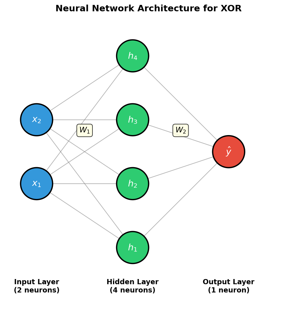
Part 1 — The architecture of a multi-layer network

A 2-2-1 network has:

• 2 inputs (x₁, x₂)
• A hidden layer of 2 neurons with sigmoid activations
• An output neuron with sigmoid activation
• 9 parameters total: 4 input→hidden weights, 2 hidden biases, 2 hidden→output weights, 1 output bias

The replacement of the step function with the sigmoid is the key. Sigmoid is smooth and differentiable everywhere; the step function is not. Gradient-based learning needs derivatives — and only continuous activations have them.

def sigmoid(z):
    return 1 / (1 + np.exp(-z))

def sigmoid_deriv(z):
    s = sigmoid(z)
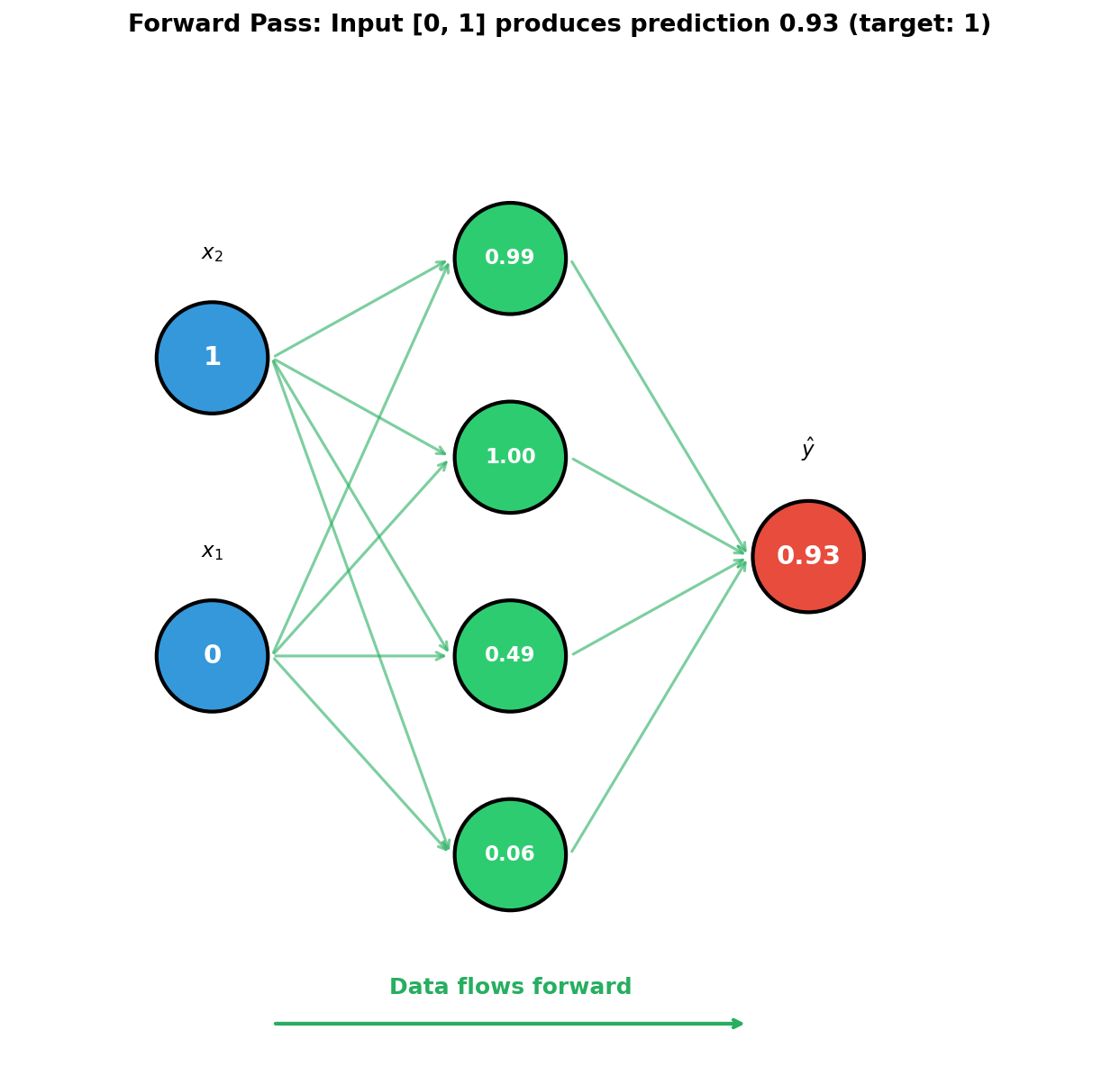
    return s * (1 - s)

Part 2 — Forward pass

Compute the hidden activations then the output:

def forward(self, x):
    z1 = W1 @ x + b1                  # hidden pre-activation
    h  = sigmoid(z1)                  # hidden activation
    z2 = W2 @ h + b2                  # output pre-activation
    y  = sigmoid(z2)                  # output activation
    return y, (z1, h, z2)             # also cache for backprop

The cache (z1, h, z2) is essential — backprop needs these values to compute derivatives without redundant recomputation.

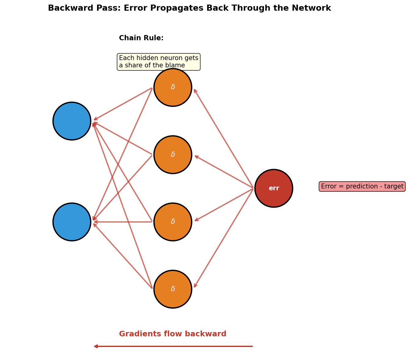
Part 3 — Backward pass via the chain rule

The loss for one training example is squared error:

L = (y_pred − y_true)²

We want ∂L/∂w for every weight w. The chain rule propagates the error backward through each operation:

def backward(self, x, y_true, cache):
    z1, h, z2 = cache
    y_pred = sigmoid(z2)

    dL_dy   = 2 * (y_pred - y_true)             # ∂L/∂y_pred
    dy_dz2  = sigmoid_deriv(z2)                 # ∂y_pred/∂z2
    dL_dz2  = dL_dy * dy_dz2                    # combine

    dL_dW2  = np.outer(dL_dz2, h)               # output weights
    dL_db2  = dL_dz2                            # output bias

    dL_dh   = W2.T @ dL_dz2                     # error at hidden activations
    dL_dz1  = dL_dh * sigmoid_deriv(z1)         # combine with sigmoid deriv

    dL_dW1  = np.outer(dL_dz1, x)               # input weights
    dL_db1  = dL_dz1                            # hidden biases

    return dL_dW1, dL_db1, dL_dW2, dL_db2

Each line is one application of the chain rule. The genius of backprop is reusing the cached forward activations to avoid recomputing them [2, 3].

Synthesis project

EXECUTE I.

Train on XOR

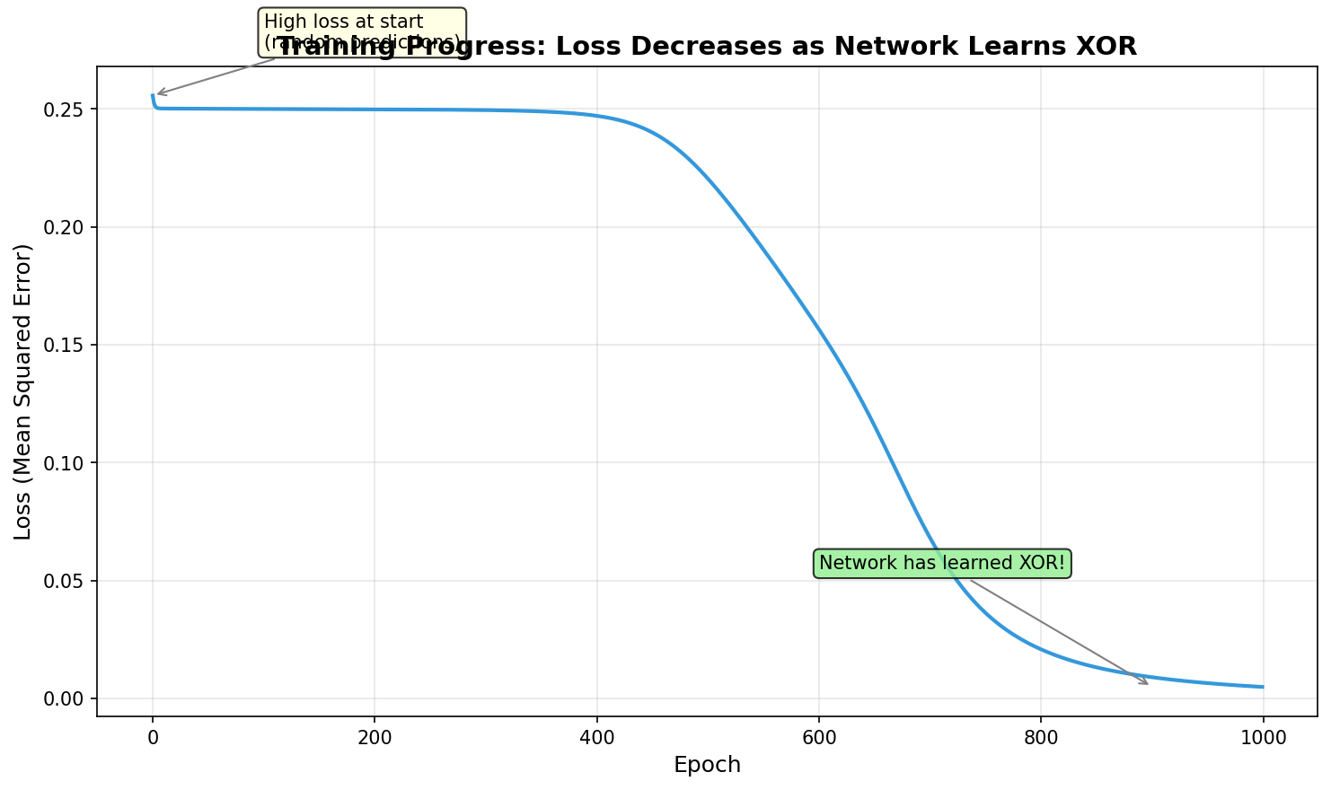
Run simple_xor_train.py. The script initialises a 2-2-1 network with random weights and trains for 5000 epochs using batch gradient descent. The script saves a sequence of decision-boundary images as training progresses.

Reflection questions

• Why does the loss curve have a long plateau near the start?
• Why is the final boundary curved, not straight?
• What happens if you initialise all weights to zero?

Answers

Plateau — at random initialisation, the sigmoid outputs are near 0.5, gradients are small, and the network needs many epochs to escape the initial flat region. This is the classic “vanishing gradient” warmup.

Curved boundary — the hidden layer transforms the 2D input space into a 2D hidden space where XOR is linearly separable. The output sigmoid draws a line in the hidden space; pulled back to the input space, that line becomes a curve.

Zero init — all hidden neurons compute identical outputs, gradients are identical, and updates are identical. The network never differentiates the hidden neurons; XOR remains unsolved. This is why neural networks always use random initialisation.

rng = np.random.default_rng(0)
N = 200
inside = rng.normal(0, 0.5, (N, 2))
outside = rng.normal(0, 1.6, (N, 2))
outside = outside[np.linalg.norm(outside, axis=1) > 1.2]
X = np.vstack([inside, outside])
y = np.concatenate([np.ones(len(inside)), np.zeros(len(outside))])

Downloads

References