9.2.3 Recurrent Networks
Process sequences with a network that has *memory* — a hidden state passed from step to step. The vanilla RNN learns to generate sequences character by character; LSTMs and Transformers are the modern descendants of the same recurrent idea.
Big question
How does a neural network handle data that arrives one item at a time, where the meaning of each item depends on what came before? Text is the canonical example: the meaning of “bank” depends on whether we previously said “river” or “money.” A feedforward network has no way to remember previous inputs. Recurrent Neural Networks (RNNs) maintain a hidden state vector that is updated at every time step, carrying information forward [1]. The vanilla RNN of 1986 became the LSTM of 1997 [2], the GRU of 2014 [3], and eventually the Transformer of 2017 [4]. The recurrent idea has evolved, but it began here.
Learning objectives
- Express an RNN as a function
h_t = tanh(W_x x_t + W_h h_{t-1} + b)that maps an input + previous state to a new state. - Unroll the recurrence in time and apply backpropagation through time (BPTT).
- Train a character-level RNN on a small text corpus and generate plausible-sounding output.
- Identify the vanishing-gradient problem that motivated LSTMs and GRUs.
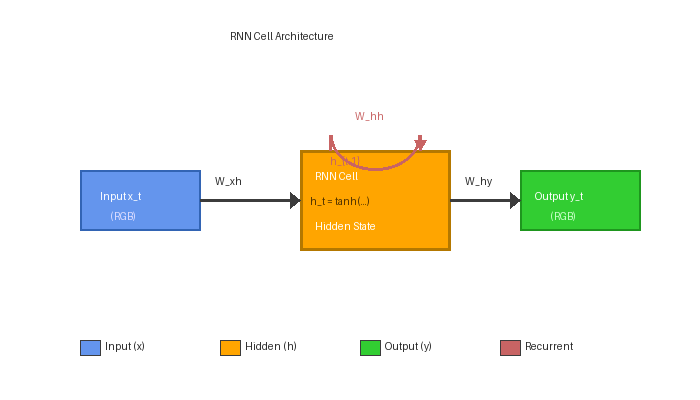
Part 1 — The recurrent unit
A vanilla RNN cell maps an input vector x_t and a previous hidden state h_{t-1} to a new hidden state:
def rnn_step(x_t, h_prev, W_x, W_h, b):
    return np.tanh(W_x @ x_t + W_h @ h_prev + b)
The same weights W_x, W_h, b are reused at every time step. Computing the output sequence is a simple loop:
def forward(self, x_seq):
    h = np.zeros(self.hidden_size)
    states = [h]
    for x_t in x_seq:
        h = rnn_step(x_t, h, self.W_x, self.W_h, self.b)
        states.append(h)
    return states
The hidden state is the network’s memory — it carries information about everything seen so far. The capacity of that memory is limited by the dimensionality of h; bigger hidden vectors hold more information [5].
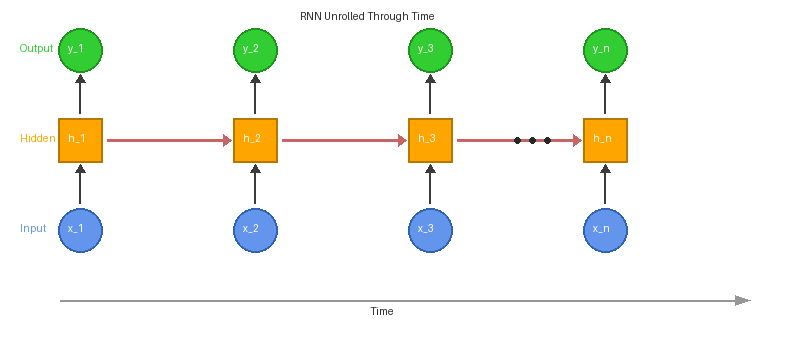
Part 2 — Unrolling and backpropagation through time
To train, we treat the RNN as a feedforward network with T layers (one per time step), all sharing the same weights. Backpropagation propagates gradients backward through every step:
∂L/∂W_h = Σ_t ∂L_t/∂h_t · ∂h_t/∂W_hThis is Backpropagation Through Time (BPTT) [1]. The catch: gradients can vanish or explode exponentially as they propagate backward through many time steps, because the same recurrence matrix W_h is multiplied repeatedly. For T = 100 steps, even a small spectral radius error compounds.
Part 3 — Character-level language model
The classic RNN demo (Karpathy 2015) is a character-level language model: input one character, predict the next. Train on Shakespeare or Linux kernel source, and the network generates eerily plausible text [6].
# Forward pass for one input character
h = rnn_step(one_hot(char), h, W_x, W_h, b)
logits = W_y @ h + b_y
probs = softmax(logits)
next_char = np.random.choice(len(vocab), p=probs)
After enough training, the network learns spelling, basic grammar, and even some style. It does not learn semantics: the output is fluent gibberish, not coherent thought.

Synthesis project
Run the char-level RNN
Run rnn_starter.py from the downloads. It trains a small RNN on a sample text corpus for 100 epochs and generates sample output every 10 epochs.
Reflection questions
- Why does early-training output look like random noise?
- After 100 epochs, the output has real words but no meaning. What is the network not learning?
- What would the same network look like on numeric time-series data (stock prices, sensor readings) instead of text?
Answers
Early output — random initialisation → softmax outputs are nearly uniform → sampling produces noise. The network needs to learn letter frequencies first, then digrams (two-letter patterns), then word-like structures.
Missing semantics — the RNN learns form (which letters follow which) but not meaning (what words refer to). It has no grounding in the world. Modern large language models learn semantics by training on far more text and on self-supervised tasks that force them to predict context, but the basic limitation remains: language models learn what looks like meaningful text, not necessarily what is meaningful.
Numeric time series — same network, different input encoding (real-valued vectors instead of one-hot characters). RNNs were the standard tool for time-series forecasting, anomaly detection, and speech recognition through the 2010s.
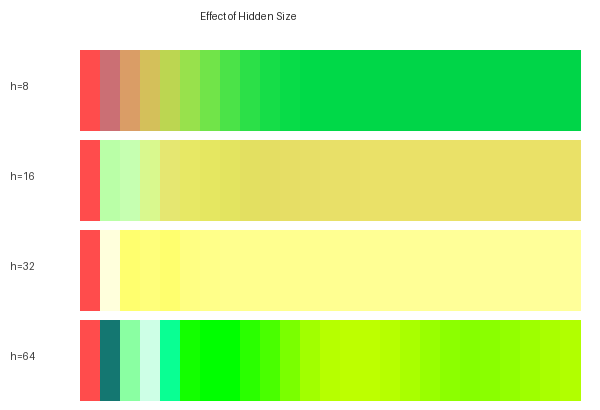
Hidden-size sweep
Train RNNs with hidden sizes 8, 64, 256 on the same corpus. Compare:
Goals
- Final training loss for each.
- Sample output quality at each.
- Wall-clock training time per epoch.
Expected outcomes
- 8 hidden: low capacity. Loss is high; samples are mostly noise.
- 64 hidden: standard. Loss is much lower; samples have word-like structure.
- 256 hidden: more capacity. Lower loss; samples have plausible sentence structure but 2-3× slower training.
The compute trade-off is fundamental: bigger hidden states give better models but quadratically more compute (recurrence is O(H²) per step).
Spot the vanishing gradient
Train an RNN on a sequence task where you must remember the first element of a long sequence to predict the last. With sequence length 5, the network learns fine. With sequence length 100, it can’t.
Task and outcome
# Task: input sequence of length T; first element is class 0 or 1;
# remaining T-1 elements are noise; predict the first element at step T.
def make_batch(T, batch_size=64):
    cls = rng.integers(0, 2, batch_size)
    xs = rng.normal(0, 1, (batch_size, T, 1))
    xs[:, 0, 0] = cls
    return xs, cls
A vanilla RNN with T = 5 learns this task in a few epochs. With T = 100, the gradient from step 100 back to step 1 has been multiplied by W_h 100 times — if its spectral radius is < 1, the gradient has vanished. The network never connects the prediction to the input. LSTMs solve this exact problem with their gating mechanism — adding gated additive updates that don’t vanish under repeated application.
Downloads
rnn_starter.py — char-level RNNReferences
- [1] Rumelhart, D. E., Hinton, G. E., & Williams, R. J. (1986). Learning representations by back-propagating errors. Nature, 323(6088), 533–536.
- [2] Hochreiter, S., & Schmidhuber, J. (1997). Long short-term memory. Neural Computation, 9(8), 1735–1780.
- [3] Cho, K., van Merriënboer, B., Gulcehre, C., et al. (2014). Learning phrase representations using RNN encoder–decoder for statistical machine translation. EMNLP, 1724–1734.
- [4] Vaswani, A., Shazeer, N., Parmar, N., et al. (2017). Attention is all you need. NeurIPS 30.
- [5] Elman, J. L. (1990). Finding structure in time. Cognitive Science, 14(2), 179–211.
- [6] Karpathy, A. (2015). The unreasonable effectiveness of recurrent neural networks. Andrej Karpathy Blog.
- [7] Devlin, J., Chang, M.-W., Lee, K., & Toutanova, K. (2019). BERT: Pre-training of deep bidirectional transformers for language understanding. NAACL-HLT, 4171–4186.