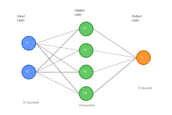
9.2.1 Feedforward Networks
Stack multiple hidden layers and discover what depth buys you over width. A 2-8-8-1 network learns curved boundaries the perceptron and shallow XOR-trainer can't, and the same architecture scales up to classify handwriting and recognise images.
Big question
If a single hidden layer can approximate any continuous function (Universal Approximation Theorem, 1989), why does anybody build deeper networks? The answer is that width and depth are different resources. A shallow but wide network needs exponentially many neurons to express the same function a deep narrow network captures in polynomially many [1]. Depth gives you compositional structure: each layer learns features built from features below. This is the central insight of modern deep learning — the network “discovers” useful intermediate representations on its own.
Learning objectives
- Generalise the 2-2-1 backprop code from 9.1.2 to a configurable layer list
[2, 8, 8, 1]. - Train a 2-8-8-1 network on non-XOR datasets (spirals, moons, concentric circles).
- Visualise hidden-layer activations as a learned representation of the input.
- Compare depth (more layers) vs width (more neurons per layer) on the same problem.
Part 1 — A configurable forward pass
The 2-2-1 network of 9.1.2 hard-coded two weight matrices. Generalise to any architecture:
class MLP:
    def __init__(self, layers, seed=0):
        rng = np.random.default_rng(seed)
        self.Ws, self.bs = [], []
        for i in range(len(layers) - 1):
            # He init for ReLU
            self.Ws.append(rng.normal(0, np.sqrt(2/layers[i]),
                                       size=(layers[i+1], layers[i])))
            self.bs.append(np.zeros(layers[i+1]))

    def forward(self, x):
        a = x
        cache = [x]
        for W, b in zip(self.Ws[:-1], self.bs[:-1]):
            z = W @ a + b
            a = np.maximum(0, z)        # ReLU hidden
            cache.append(a)
        # final layer with sigmoid for binary classification
        z = self.Ws[-1] @ a + self.bs[-1]
        y = 1 / (1 + np.exp(-z))
        cache.append(y)
        return y, cache
layers=[2, 8, 8, 1] gives a 2-input, two-hidden-layer, 1-output network with 8 neurons each in the hidden layers.
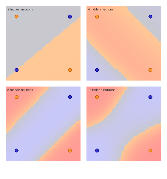
Part 2 — Depth as composition
Each hidden layer applies its own non-linear transformation. The first hidden layer carves the input space into half-spaces (just like a perceptron); the second hidden layer combines those half-spaces into more complex regions; and so on. With ReLU activations, each additional layer can roughly double the number of linear regions the network expresses [2].
Part 3 — Learned representations
The hidden activations are the learned representation. For a 2-8-8-1 network trained on a spiral dataset, plotting the 8-dimensional hidden activations (projected to 2D via PCA) reveals that the network has un-twisted the spiral — in hidden space the two classes are linearly separable, exactly the property the output layer needs.
Synthesis project
Train on the spiral dataset
Run feedforward_network.py from the downloads. It generates two interlocked spirals, trains a 2-8-8-1 MLP for 3000 epochs, and saves the decision-boundary plot.
Reflection questions
- The spiral dataset is harder than XOR. What makes it harder, exactly?
- Why does the boundary converge from a straight-line approximation to a curve as training progresses?
- What would the network look like if you only had 2 hidden neurons in both layers?
Answers
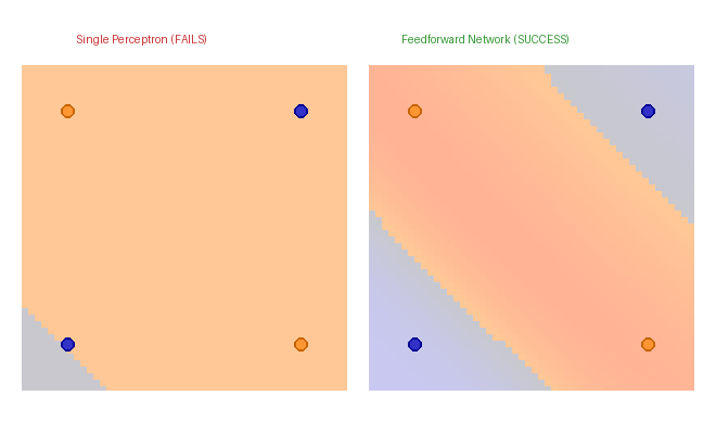
Spiral difficulty — XOR has 4 points and is finite. Spirals are continuous interleaved curves; the network must approximate a very curvy decision boundary with finitely many neurons. More expressive architecture is required.
Convergence — early in training, ReLU activations are near-linear; the network behaves like a single linear unit. As gradients accumulate, ReLU’s “kinks” position themselves to carve out the spiral shape. Each kink in the final boundary is one ReLU activation switching from 0 to positive somewhere in input space.
2 hidden / 2 hidden — the network barely has enough capacity. With ReLU you’d get a piecewise-linear boundary that approximates the spiral roughly. Bumping the width is what gives you smoothness.
Width vs depth experiment
Train three networks on the same spiral data and compare their final loss:
Goals
- Shallow & wide —
[2, 64, 1]. One hidden layer, 64 neurons. - Standard —
[2, 8, 8, 1]. Two hidden layers, 8 each. - Deep & narrow —
[2, 4, 4, 4, 4, 1]. Four hidden layers, 4 each.
Expected outcomes
All three reach low loss given enough epochs, but with different training characteristics:
- Shallow wide: trains fastest per epoch (fewer layers = less backprop computation). Boundary is smooth.
- Standard: slightly slower per epoch; reaches similar quality.
- Deep narrow: hardest to train. Without batch normalisation or residual connections, the deeper network may struggle with gradient flow. When it works, the boundary has noticeably more compositional structure.
Decision-boundary evolution GIF
Generate a sequence of decision-boundary images at epochs 0, 100, 300, 1000, 3000, and assemble into a GIF showing the network’s learning trajectory.
Implementation hint
import imageio

frames = []
for epoch in [0, 100, 300, 1000, 3000]:
    train_until(net, X, y, epoch)
    img = render_boundary(net)
    frames.append(img)
imageio.mimsave('evolution.gif', frames, fps=2)
The fun of this exercise is watching the boundary morph. Networks don’t go directly from “flat” to “perfect” — they hit recognisable intermediate stages: a single dividing line, a more complex curve, the rough spiral shape, then refinement.
Downloads
feedforward_network.py — train + visualise feedforward_starter.py — Exercise starterReferences
- [1] Telgarsky, M. (2016). Benefits of depth in neural networks. Conference on Learning Theory (COLT).
- [2] Montufar, G. F., Pascanu, R., Cho, K., & Bengio, Y. (2014). On the number of linear regions of deep neural networks. NeurIPS 27.
- [3] Cybenko, G. (1989). Approximation by superpositions of a sigmoidal function. Mathematics of Control, Signals, and Systems, 2(4), 303–314.
- [4] He, K., Zhang, X., Ren, S., & Sun, J. (2015). Delving deep into rectifiers. ICCV, 1026–1034.
- [5] Goodfellow, I., Bengio, Y., & Courville, A. (2016). Deep Learning. MIT Press.
- [6] LeCun, Y., Bengio, Y., & Hinton, G. (2015). Deep learning. Nature, 521(7553), 436–444.