9.1.3 Activation Functions as Art
Visualise the seven canonical activation functions — sigmoid, tanh, ReLU, leaky ReLU, ELU, GELU, Swish — and feed an image through each. The choice of activation is one of the few decisions that hasn't moved in a decade.
Big question
What does the activation function actually do? Without it, a neural network is just a stack of linear transforms — and any stack of linear transforms collapses into a single linear transform [1]. The activation introduces non-linearity, the one ingredient that lets the network learn curved decision boundaries, image features, and language structure. Choosing the activation function is one of the few neural-network decisions where the field has reached near-consensus: ReLU (or its variants) dominate, with sigmoid and tanh largely retired to recurrent networks and output layers [2].
Learning objectives
- Plot the curve and derivative of each canonical activation function.
- Explain why ReLU (
max(0, x)) became standard around 2012 — sparsity, no saturation, fast gradient. - Apply each activation pixel-wise to an image and observe how it transforms the value distribution.
- Connect the activation choice to the vanishing gradient problem in deep networks.
Part 1 — Why non-linearity matters
Without an activation, a multi-layer network reduces to a single matrix multiplication:
y = W₃ (W₂ (W₁ x)) = (W₃ W₂ W₁) x = W' xThe composition of linear functions is linear. To learn anything more interesting than a hyperplane separator, you need a non-linear function between layers. Any non-linear function works in principle; in practice, the seven canonical activations balance three concerns:
- Differentiability — for backpropagation.
- Saturation — sigmoid and tanh squash inputs into bounded ranges, which causes gradients to vanish for large
|x|. - Computational cost —
max(0, x)is one comparison;tanh(x)is several transcendental operations.
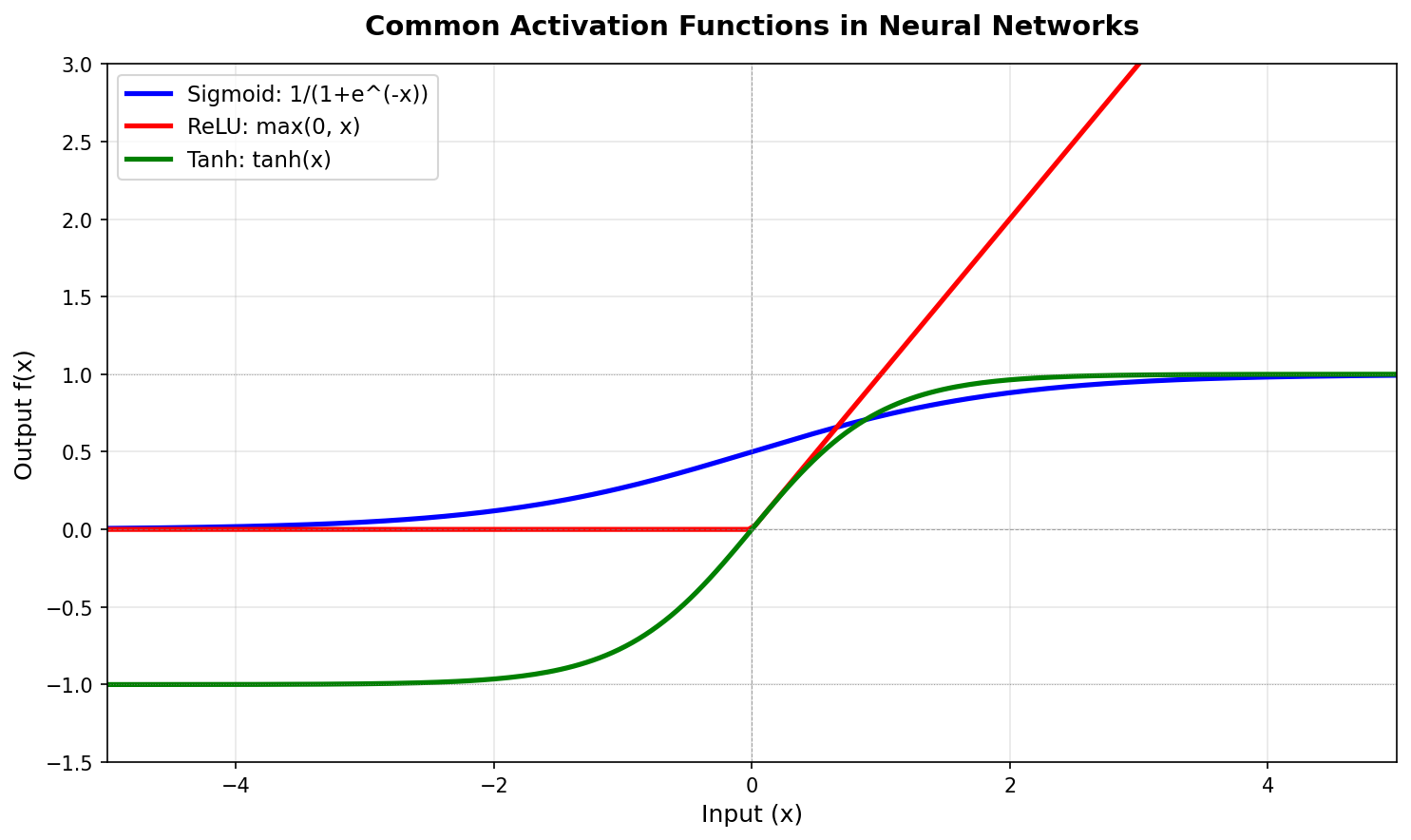
Part 2 — The canonical functions
import numpy as np

def sigmoid(x):     return 1 / (1 + np.exp(-x))
def tanh(x):        return np.tanh(x)
def relu(x):        return np.maximum(0, x)
def leaky_relu(x, alpha=0.01): return np.where(x > 0, x, alpha * x)
def elu(x, alpha=1.0): return np.where(x > 0, x, alpha * (np.exp(x) - 1))
def gelu(x):        return 0.5 * x * (1 + np.tanh(np.sqrt(2/np.pi) * (x + 0.044715 * x**3)))
def swish(x):       return x * sigmoid(x)
The historical sequence is instructive:
| Function | Year | Notes |
|---|---|---|
| Sigmoid | 1958 | Smooth, but saturates → vanishing gradients in deep nets |
| Tanh | 1980s | Zero-centred sigmoid; better for backprop but still saturates |
| ReLU | 2010 | One comparison; no saturation for x > 0. Default for CNNs by 2012 [3] |
| Leaky ReLU | 2013 | Tiny negative slope to fix the “dying ReLU” problem |
| ELU | 2015 | Smoother negative branch via exp |
| GELU | 2016 | Stochastic + smooth; default in transformers [4] |
| Swish | 2017 | x · sigmoid(x); found by neural architecture search |
The ReLU paper of Glorot, Bordes & Bengio (2011) was the inflection point — ReLU-based networks trained faster and reached lower loss than sigmoid networks, on the same data and architecture. By 2012’s AlexNet, ReLU was standard [3, 5].
Part 3 — Apply each to an image
A useful way to see what each activation does is to apply it pixel-wise to a normalised image. The transformations are striking:
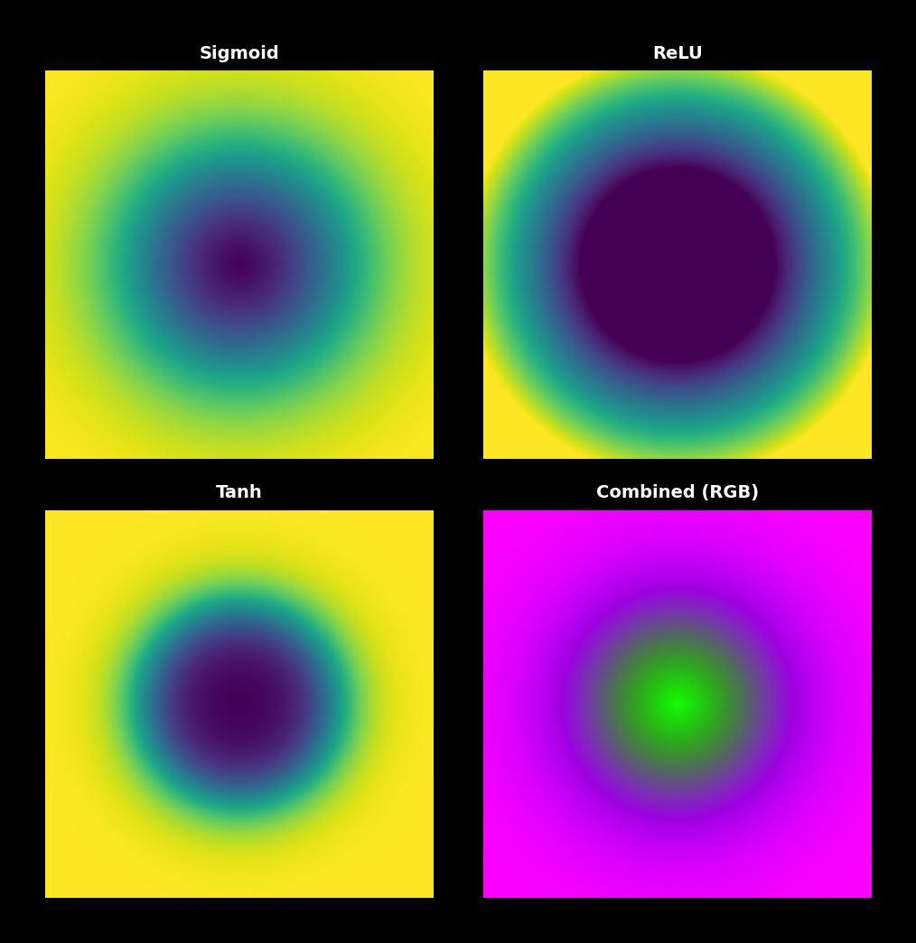
The effect on real images:
- Sigmoid — compresses everything into the middle of the brightness range. The image looks low-contrast.
- Tanh — same shape, signed. Slightly more contrast than sigmoid.
- ReLU — anything below zero (after centring) → black. Sharp half-clip effect.
- Leaky ReLU — same as ReLU but with very dim negatives instead of pure black.
- ELU — like leaky ReLU but with smoother negative tail.
- GELU/Swish — a tiny negative slope that grows smoothly into positive identity. Hard to distinguish visually from ReLU at first glance, but training dynamics differ.
Synthesis project
Plot all activations and their derivatives
Run activation_functions_art.py. The script plots all seven functions on a shared axis and their derivatives separately.
Reflection questions
- Which activations saturate (have near-zero derivatives for large
|x|)? - Why does saturation cause the “vanishing gradient” problem in deep networks?
- Which activations are not zero-centred? Why does that matter?
Answers
Saturation — sigmoid and tanh both flatten at extremes; their derivatives → 0 as |x| → ∞. ReLU saturates only on the negative side (derivative is exactly 0 there); the positive side has derivative 1 forever.
Vanishing gradient — backprop multiplies derivatives through layers. If each derivative is < 1, the product shrinks exponentially with depth. After 5–10 sigmoid layers, gradients are too small to update earlier weights. This is why deep sigmoid networks were untrainable before ReLU.
Zero-centring — sigmoid outputs are in (0, 1), so the mean of activations is positive. This biases the gradient sign on subsequent layers, slowing training. Tanh, GELU, and Swish are zero-centred and converge faster as a result.
Apply activations to an image
Edit activation_starter.py to apply each activation to a normalised input image and save a 7-panel comparison.
Goals
- Normalise the image to
[-2, 2]before applying — gives the non-linearities room to show their shape. - Apply each function pixel-wise.
- Stack into a 2×4 grid with the original in the first slot for reference.
Expected visual result
You’ll see distinct visual signatures:
- Sigmoid panel looks washed-out (compressed range).
- ReLU panel has half the image pure black.
- Tanh / GELU / Swish panels look closest to the original.
The exercise mirrors what activation functions do inside the network between layers — each step of forward propagation reshapes the activation distribution.
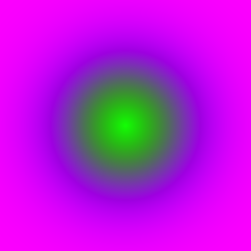
Aurora — the activation as art
Build an artistic composition using activation functions: generate a smooth field (e.g. fbm noise from Module 06), apply different activations to different regions, and combine into one image.

Approach
import numpy as np
# (assume fbm() helper available from Module 6)

H, W = 400, 800
noise = fbm((H, W), scale=120, octaves=6)
noise = (noise - 0.5) * 4   # centre around 0 with width

# Apply tanh to make smooth banded structure
shaped = np.tanh(noise * 2)

# Map to colour
rgb = np.zeros((H, W, 3))
rgb[..., 0] = np.clip(shaped * 0.3 + 0.2, 0, 1)
rgb[..., 1] = np.clip(shaped * 0.8 + 0.4, 0, 1)
rgb[..., 2] = np.clip(0.6 + shaped * 0.3, 0, 1)
The activation is the artistic knob: tanh gives smooth bands; ReLU gives sharp half-bands; sigmoid gives soft horizons. Each gives a different aurora-like aesthetic.
Downloads
activation_functions_art.py — plot curves activation_starter.py — apply to images challenge_aurora.py — aurora referenceReferences
- [1] Goodfellow, I., Bengio, Y., & Courville, A. (2016). Deep Learning. MIT Press.
- [2] LeCun, Y., Bengio, Y., & Hinton, G. (2015). Deep learning. Nature, 521(7553), 436–444.
- [3] Glorot, X., Bordes, A., & Bengio, Y. (2011). Deep sparse rectifier neural networks. Proceedings of AISTATS, 15, 315–323.
- [4] Hendrycks, D., & Gimpel, K. (2016). Gaussian Error Linear Units (GELUs). arXiv:1606.08415.
- [5] Krizhevsky, A., Sutskever, I., & Hinton, G. E. (2012). ImageNet classification with deep convolutional neural networks. NeurIPS 25, 1097–1105.
- [6] He, K., Zhang, X., Ren, S., & Sun, J. (2015). Delving deep into rectifiers: Surpassing human-level performance on ImageNet classification. ICCV, 1026–1034.
- [7] Ramachandran, P., Zoph, B., & Le, Q. V. (2017). Searching for activation functions. arXiv:1710.05941.