9.2.2 Convolutional Networks
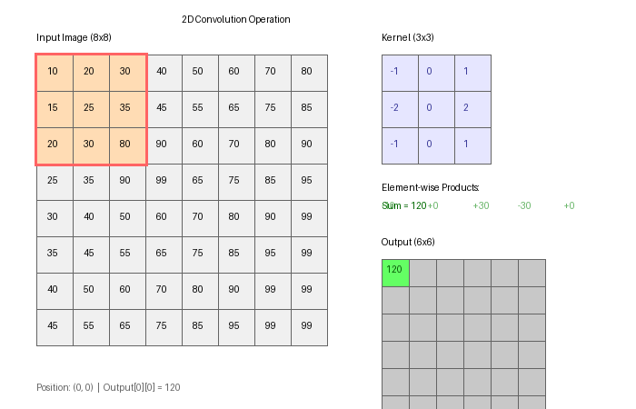
Replace fully-connected layers with convolutions: shared weights that slide across the image. The same trick used as a kernel in 3.4.1 becomes the central operation of every computer-vision network from LeNet (1998) to today.
Big question
Why don’t we just use a giant feedforward network on images? A 224×224 RGB image has 150,528 input pixels. A single fully-connected hidden layer with 1000 neurons would have 150 million weights — for one layer. Most of those weights would learn redundant local-pattern detectors for every pixel position. Yann LeCun’s insight in 1989 was that the same edge detector should work at every location: share the weights across positions. The convolutional layer is born — a tiny 3×3 or 5×5 filter, slid across the image, learning one feature detector that runs everywhere [1, 2]. This single architectural idea is what made computer-vision deep learning practical.
Learning objectives
- Connect convolution-as-kernel (3.4.1) to convolution-as-CNN-layer — same math, learned weights.
- Implement a forward convolution in NumPy and apply learned filters to an image.
- Understand the CNN architecture: convolution → activation → pooling, stacked.
- Visualise feature maps — the per-filter response at each layer — to see what the network is “looking at.”
Part 1 — Shared weights, sliding filters
A fully-connected layer treats every pixel as an independent input feature: weights w(i, j) connect input pixel (i, j) to every hidden neuron. A convolutional layer shares weights across positions: one 3×3 filter is applied at every location of the input.
def conv2d(image, kernel, stride=1, pad='same'):
    H, W = image.shape
    k = kernel.shape[0]
    if pad == 'same':
        p = k // 2
        image = np.pad(image, p, mode='edge')
    out = np.zeros((H, W))
    for y in range(H):
        for x in range(W):
            out[y, x] = np.sum(image[y:y+k, x:x+k] * kernel)
    return out
This is the same convolution as 3.4.1. The difference in a CNN: the kernel weights are learned by backpropagation rather than hand-designed [3].
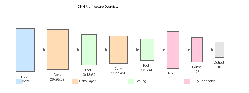
Part 2 — Convolutional layer ingredients
A practical convolutional layer has four ingredients:
- Filters —
Kfilters of shape(k, k, C_in)produceKoutput channels. - Stride — step size when sliding the filter. Stride=1 keeps spatial size; stride=2 halves it.
- Padding —
samekeeps the output size equal to input;validshrinks byk-1. - Activation — typically ReLU, applied element-wise after convolution.
out_height = (in_height - kernel + 2*pad) / stride + 1After the convolution + activation, a max-pooling layer reduces spatial size by taking the maximum over each 2×2 block. Pooling is what gives CNNs their translation invariance — the same feature at a slightly different position still fires the same downstream units [4].
Part 3 — Feature maps
After applying K filters, you have K feature maps — each one a 2D image showing where that filter “fires.” Visualising these is how you build intuition about what a CNN has learned.
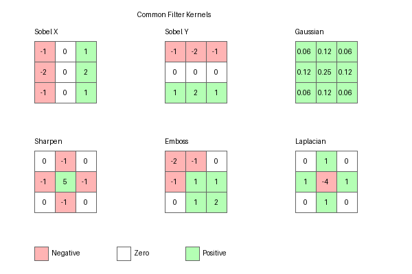
Astonishingly, early-layer filters in trained CNNs look like Gabor filters — the same oriented-edge detectors that the 1980s computer-vision community had already designed by hand. The network rediscovers these features from scratch, by gradient descent on a classification objective [2, 5].
Synthesis project
Apply learned filters to an image
Run cnn_visualization.py from the downloads. It loads pre-trained filter kernels (Sobel-like horizontal, Sobel-like vertical, blob detector, sharpening, blur), applies each to an input image, and saves the feature maps.
Reflection questions
- Each feature map is a 2D image. What do bright pixels in the feature map mean?
- The Sobel-horizontal filter is hand-designed in 3.4.1. Why does a CNN trained on image classification learn something nearly identical in its first layer?
- What happens if you apply multiple convolutional layers to the same input?
Answers
Bright pixel = high response — that pixel’s receptive field (the patch of input the filter saw) matches what the filter is looking for. A horizontal-edge filter has bright pixels where the input has horizontal edges.
Why CNN learns Sobel — Sobel filters are optimal for detecting edges, and edges are useful features for classifying objects. Gradient descent on a classification loss naturally rediscovers useful low-level features.
Multiple layers — early layers detect edges, middle layers detect parts (corners, textures, shape fragments), late layers detect whole objects. This hierarchy is what gives CNNs their power and what made deep learning “the deeper the better” in the 2010s.
Artistic filters via convolution
Apply each of these hand-crafted kernels to an image and observe the artistic effects:
Goals
- Edge detection — Sobel kernels (3.4.2) for grayscale outline.
- Emboss —
[[-2, -1, 0], [-1, 1, 1], [0, 1, 2]]for 3D-looking shading. - Sharpen —
[[0, -1, 0], [-1, 5, -1], [0, -1, 0]]for crisp detail.
Implementation
Same conv2d from Part 1. Apply each filter; save the result. The emboss filter is asymmetric (the sum is non-zero) so the output has a directional shading effect — a kind of pseudo-3D look.
Build a tiny CNN forward pass
Implement a 2-conv-layer CNN forward pass in NumPy. Input is a 28×28 image (MNIST-style); the network has:
- Conv layer 1: 4 filters of size 3×3, stride 1, ReLU.
- Max-pool: 2×2, stride 2.
- Conv layer 2: 8 filters of size 3×3, stride 1, ReLU.
- Max-pool: 2×2, stride 2.
- Output: flatten → 1 dense layer.
import numpy as np

def conv2d(x, W, b, stride=1):
    """Multi-filter 2D convolution with bias.
    x: (H, W, C_in), W: (K, k, k, C_in), b: (K,)
    Returns: (H_out, W_out, K)
    """
    H, W_in, C = x.shape
    K, kh, kw, _ = W.shape
    # TODO: implement using nested loops or im2col.

def maxpool2d(x, size=2, stride=2):
    """2x2 max pool with stride 2."""
    # TODO

def relu(x):
    return np.maximum(0, x)

# Build the network
def forward(image):
    x = image[..., None]                # (28, 28, 1)
    x = relu(conv2d(x, W1, b1))         # (28, 28, 4)
    x = maxpool2d(x)                    # (14, 14, 4)
    x = relu(conv2d(x, W2, b2))         # (14, 14, 8)
    x = maxpool2d(x)                    # (7, 7, 8)
    x = x.flatten()
    return W3 @ x + b3                  # logits
Approach
You’re rebuilding LeNet’s first half. The convolution implementation in pure Python is slow (O(K · k² · H · W)); production frameworks use im2col to express it as a matrix multiply that benchmarks fast on BLAS. The point of this exercise isn’t performance — it’s seeing the full forward pass spelled out so you can map every operation to a Python line.
Downloads
cnn_visualization.py — apply learned filters cnn_starter.py — tiny CNN forward passReferences
- [1] LeCun, Y., Boser, B., Denker, J. S., et al. (1989). Backpropagation applied to handwritten zip code recognition. Neural Computation, 1(4), 541–551.
- [2] LeCun, Y., Bottou, L., Bengio, Y., & Haffner, P. (1998). Gradient-based learning applied to document recognition. Proceedings of the IEEE, 86(11), 2278–2324.
- [3] Goodfellow, I., Bengio, Y., & Courville, A. (2016). Deep Learning. MIT Press.
- [4] Boureau, Y.-L., Ponce, J., & LeCun, Y. (2010). A theoretical analysis of feature pooling in visual recognition. ICML 27.
- [5] Zeiler, M. D., & Fergus, R. (2014). Visualizing and understanding convolutional networks. ECCV, 818–833.
- [6] Krizhevsky, A., Sutskever, I., & Hinton, G. E. (2012). ImageNet classification with deep convolutional neural networks. NeurIPS 25, 1097–1105.
- [7] He, K., Zhang, X., Ren, S., & Sun, J. (2016). Deep residual learning for image recognition. CVPR, 770–778.