4.1.3 Mandelbrot Set

Overview

The Mandelbrot set is the most famous fractal in mathematics, but the rule that produces it is almost embarrassingly short: at every step, replace $z$ with $z$-squared plus $c$. For each point $c$ in the complex plane, start with $z_0 = 0$ and iterate. If the orbit stays bounded forever, $c$ belongs to the set; if it shoots off to infinity, $c$ is outside. Colour each pixel by how fast it escapes and the result is the iconic cardioid-and-bulbs silhouette with an infinitely complex boundary that Benoit Mandelbrot first rendered at IBM in 1980 [1].

This is the first lesson in Module 04 where the recursion lives inside the algorithm rather than inside the function call stack. The dragon curve (4.1.2) built a string by recursing in Python; the Mandelbrot iteration runs the same arithmetic on every pixel of a 512×512 grid in parallel using NumPy. Iteration replaces recursion when you need millions of evaluations.

Learning objectives

1. Build a 2D grid of complex numbers with np.meshgrid and 1j.
2. Implement the escape-time algorithm vectorised over the whole grid with a boolean mask.
3. Map escape iteration counts to colours and recognise why $|z| > 2$ is the right threshold.
4. Connect the Mandelbrot iteration to the quadratic map $z^2 + c$ as a dynamical system — set up for Julia sets (4.1.4) where the same map runs with a fixed $c$.

Quick start — generate the set

import numpy as np
from PIL import Image

# 1. Grid of complex numbers covering the classic Mandelbrot viewport
x = np.linspace(-2.5, 1.0, 512)
y = np.linspace(-1.5, 1.5, 512)
real, imag = np.meshgrid(x, y)
c = real + 1j * imag

# 2. Iterate z = z^2 + c, tracking how long each point survives
z = np.zeros_like(c)
iterations = np.zeros(c.shape, dtype=np.int32)
for _ in range(100):
    bounded = np.abs(z) <= 2
    z[bounded] = z[bounded]**2 + c[bounded]
    iterations[bounded] += 1

# 3. Map iteration counts to a grayscale image
gray = (iterations / 100 * 255).astype(np.uint8)
Image.fromarray(gray).save('mandelbrot_basic.png')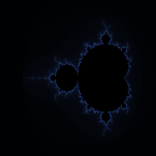

Core concepts

Concept 1 — Complex numbers as pixel coordinates

A complex number $c = a + bi$ has a real part $a$ and an imaginary part $b$, where $i$ is the square root of $-1$. Geometrically, $c$ is a point in a 2D plane: $a$ is the horizontal coordinate, $b$ the vertical. The Mandelbrot iteration runs on that 2D plane, so the very first thing you do is build a grid of complex numbers — one per pixel in the output image.

NumPy makes the grid in three lines:

real_values = np.linspace(-2.5, 1.0, 512)   # horizontal axis
imag_values = np.linspace(-1.5, 1.5, 512)   # vertical axis
real, imag = np.meshgrid(real_values, imag_values)
c = real + 1j * imag                          # 512×512 complex grid

meshgrid broadcasts the two 1D axes into matching 2D grids; 1j is Python’s syntax for the imaginary unit. Each entry c[i, j] is the complex number for the pixel at row i, column j. Change the bounds in np.linspace and you zoom into a different region of the plane — the cleanest of all viewport controls.

Concept 2 — The escape-time algorithm

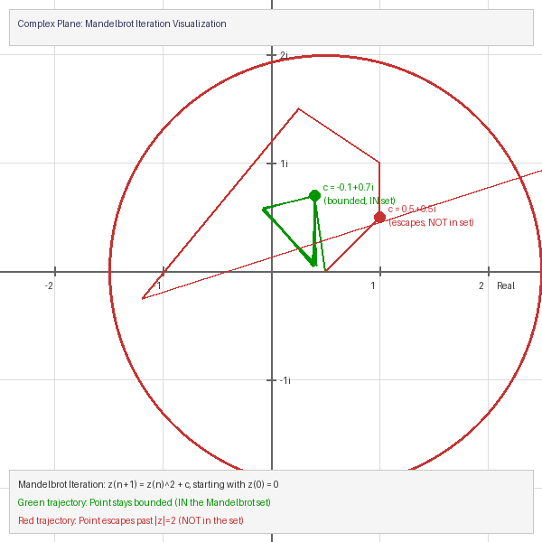
The Mandelbrot iteration is one line of arithmetic — the next value of $z$ equals the current $z$ squared, plus $c$, starting from $z_0 = 0$:

$z$-next $= z^2 + c$, with $z_0 = 0$.

For a fixed $c$, you run this repeatedly. Two things can happen:

• The orbit stays bounded — $|z_n|$ never exceeds 2 — and we say $c$ belongs to the Mandelbrot set.
• The orbit escapes — $|z_n| > 2$ for some $n$ — and we say $c$ is outside the set.

The cut-off at $|z| > 2$ is not arbitrary: once $|z|$ crosses 2, the next iteration squares it (so $|z|$ doubles roughly), and the orbit is guaranteed to run away to infinity [3]. So 2 is the escape threshold for free.

The vectorised version runs the same arithmetic on every grid point in parallel, masking out the points that have already escaped so they no longer participate:

z = np.zeros_like(c, dtype=np.complex128)
iterations = np.zeros(c.shape, dtype=np.int32)

for _ in range(max_iterations):
    bounded = np.abs(z) <= 2                       # boolean mask
    z[bounded] = z[bounded] ** 2 + c[bounded]      # update only survivors
    iterations[bounded] += 1                       # count survival

After the loop, iterations[i, j] records how many steps the orbit at pixel (i, j) survived. Points still bounded after max_iterations have iterations == max_iterations — treat them as “in the set.” Everything else escaped, and the count records when.

Concept 3 — Colour from iteration count

Once you have iterations you can paint the picture however you like. The pedagogically clearest mapping is a linear ramp from the iteration count to a colour channel:

normalized = iterations / max_iterations          # 0..1 array
image = np.zeros((height, width, 3), dtype=np.uint8)

outside = iterations < max_iterations             # the fringe
image[outside, 0] = (normalized[outside] * 80).astype(np.uint8)   # red
image[outside, 1] = (normalized[outside] * 150).astype(np.uint8)  # green
image[outside, 2] = (normalized[outside] * 255).astype(np.uint8)  # blue

# Points in the set: black
image[~outside] = [0, 0, 0]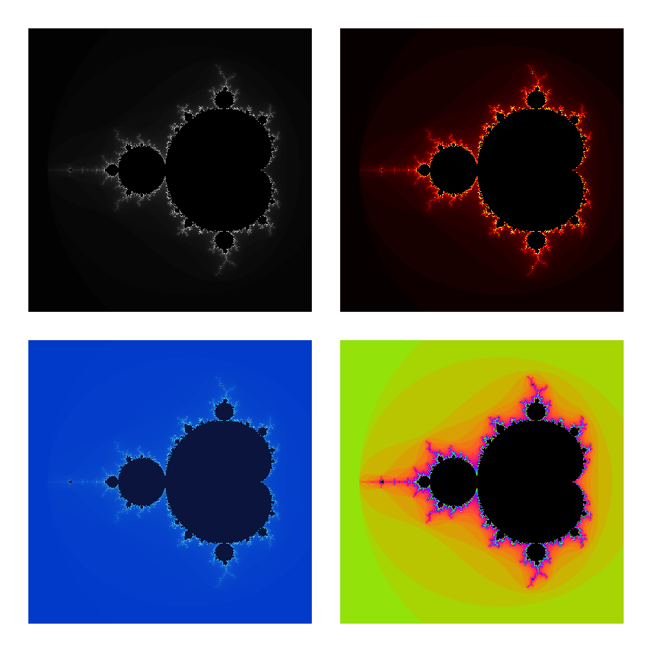

The same iterations array can be coloured with cyclic palettes (np.sin(norm * k) with phase offsets per channel) for high-contrast bands, or with a smooth matplotlib colormap like 'twilight'. The colour is a render decision; the mathematics is in iterations.

Exercises

Three exercises in Execute → Modify → Create order: run the basic Mandelbrot, retune the viewport and palette, then wrap the whole pipeline in a reusable mandelbrot_zoom function.

MODIFY II.

Zoom and recolour

Edit mandelbrot_set.py to produce three variants. Only the viewport and colour-mapping lines need to change.

Goals

1. Seahorse Valley. Zoom into the famous “seahorse valley” centred at $(-0.745, 0.113)$. Use x_min, x_max = -0.8, -0.69 and y_min, y_max = 0.05, 0.16. Raise max_iterations to at least 200 so the fine detail resolves.
2. Fire palette. Replace the blue gradient with red→orange→yellow. Drop the blue channel, raise red, keep green moderate.
3. High-resolution print. Bump the canvas to 1024×1024 — same viewport, four times as many pixels. Tip: this needs no algorithmic change, only the width and height constants.

Goal 1 — what to expect

A field of “seahorses” — paired spirals all curling the same way, separated by thin necks. The seahorse fringe is one of the most-cited regions of the set because the detail is dense enough to be visually striking at any zoom level, but the iteration count required to resolve it stays manageable.

Goal 2 — what to expect

image[outside, 0] = (normalized[outside] * 255).astype(np.uint8)  # full red
image[outside, 1] = (normalized[outside] * 150).astype(np.uint8)  # mid green
image[outside, 2] = (normalized[outside] * 30).astype(np.uint8)   # almost no blue

The escape fringe glows from dark red at the boundary through orange to yellow at the edges. Visually identical to the blue version in structure; just a different temperature.

Goal 3 — what to expect

Quadruple the pixel count, same viewport. The silhouette is unchanged; the boundary just gets crisper. Memory cost is 4× and runtime is 4× because every iteration step is now operating on 4× the pixels — but it is all still vectorised, so no algorithm change is needed.

import numpy as np
from PIL import Image

def mandelbrot_zoom(center_x, center_y, zoom_level, size=512, max_iter=200):
    """Generate a Mandelbrot image at the specified location and zoom."""
    # TODO 1: compute x_min, x_max, y_min, y_max from centre + zoom
    #         baseline viewport is roughly 3.5 wide and 3.0 tall

    # TODO 2: build the complex grid (np.linspace + meshgrid + 1j)

    # TODO 3: run the escape-time iteration loop

    # TODO 4: map iterations to colour and return an RGB array
    pass

if __name__ == '__main__':
    img = mandelbrot_zoom(-0.745, 0.113, zoom_level=50, max_iter=300)
    Image.fromarray(img).save('my_zoom.png')

x_range = 3.5 / zoom_level
y_range = 3.0 / zoom_level
x_min, x_max = center_x - x_range/2, center_x + x_range/2
y_min, y_max = center_y - y_range/2, center_y + y_range/2

real = np.linspace(x_min, x_max, size)
imag = np.linspace(y_min, y_max, size)
real_grid, imag_grid = np.meshgrid(real, imag)
c = real_grid + 1j * imag_grid

z = np.zeros_like(c)
iterations = np.zeros(c.shape, dtype=np.int32)
for _ in range(max_iter):
    bounded = np.abs(z) <= 2
    z[bounded] = z[bounded]**2 + c[bounded]
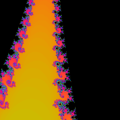
    iterations[bounded] += 1

norm = iterations / max_iter
outside = iterations < max_iter
image = np.zeros((size, size, 3), dtype=np.uint8)
image[outside, 0] = (128 + 127*np.sin(norm[outside]*10 + 0)).astype(np.uint8)
image[outside, 1] = (128 + 127*np.sin(norm[outside]*10 + 2)).astype(np.uint8)
image[outside, 2] = (128 + 127*np.sin(norm[outside]*10 + 4)).astype(np.uint8)

import numpy as np
from PIL import Image

def mandelbrot_zoom(center_x, center_y, zoom_level, size=512, max_iter=200):
    x_range = 3.5 / zoom_level
    y_range = 3.0 / zoom_level
    x_min, x_max = center_x - x_range/2, center_x + x_range/2
    y_min, y_max = center_y - y_range/2, center_y + y_range/2

    real = np.linspace(x_min, x_max, size)
    imag = np.linspace(y_min, y_max, size)
    real_grid, imag_grid = np.meshgrid(real, imag)
    c = real_grid + 1j * imag_grid

    z = np.zeros_like(c)
    iterations = np.zeros(c.shape, dtype=np.int32)
    for _ in range(max_iter):
        bounded = np.abs(z) <= 2
        z[bounded] = z[bounded]**2 + c[bounded]
        iterations[bounded] += 1

    norm = iterations / max_iter
    outside = iterations < max_iter
    image = np.zeros((size, size, 3), dtype=np.uint8)
    image[outside, 0] = (128 + 127*np.sin(norm[outside]*10 + 0)).astype(np.uint8)
    image[outside, 1] = (128 + 127*np.sin(norm[outside]*10 + 2)).astype(np.uint8)
    image[outside, 2] = (128 + 127*np.sin(norm[outside]*10 + 4)).astype(np.uint8)
    return image

if __name__ == '__main__':
    Image.fromarray(mandelbrot_zoom(-0.745, 0.113, 50, max_iter=300)).save('my_zoom.png')

Downloads

Summary

Common pitfalls to avoid

• Looping over pixels. A Python for loop over the grid is hundreds of times slower than vectorised NumPy. Always operate on the whole grid with masks.
• Forgetting the bounded mask. If you compute z**2 + c for already-escaped points, z overflows to inf and then to nan, which propagate and ruin the iteration counts.
• Underiterating at zoom. Deep zooms need more iterations to resolve the boundary. Rule of thumb: double max_iter whenever zoom passes a factor of 10.
• Hard-coding dtype=float64 for z. It silently kills the imaginary part. Use np.zeros_like(c) to inherit the dtype.

References

- [1] Mandelbrot, B. B. (1982). The Fractal Geometry of Nature. W. H. Freeman. ISBN 978-0-7167-1186-5.
- [2] Devaney, R. L. (1989). An Introduction to Chaotic Dynamical Systems (2nd ed.). Addison-Wesley. ISBN 978-0-8133-4085-2.
- [3] Peitgen, H.-O., & Richter, P. H. (1986). The Beauty of Fractals: Images of Complex Dynamical Systems. Springer-Verlag. doi:10.1007/978-3-642-61717-1
- [4] Milnor, J. (2006). Dynamics in One Complex Variable (3rd ed.). Princeton University Press. ISBN 978-0-691-12488-9.
- [5] Gleick, J. (1987). Chaos: Making a New Science. Viking Press. ISBN 978-0-14-009250-9.
- [6] Ewing, J. H., & Schober, G. (1992). The area of the Mandelbrot set. Numerische Mathematik, 61(1), 59–72. doi:10.1007/BF01385497
- [7] Harris, C. R., Millman, K. J., van der Walt, S. J., et al. (2020). Array programming with NumPy. Nature, 585, 357–362. doi:10.1038/s41586-020-2649-2