4.2.1 Fractal Trees

Overview

Trees are the natural-world poster child for fractal geometry. The trunk splits into branches, each branch splits into smaller branches, each twig terminates in still-smaller twigs — and at every scale the geometry looks similar. Mandelbrot devoted a chapter of The Fractal Geometry of Nature to this exact observation [1]. The reason is not just aesthetic: fractal branching solves a real engineering problem — maximise leaf-surface exposure to sunlight, distribute water through xylem, and stay mechanically stable — with a tiny ruleset, which is why evolution rediscovered it independently in plants, rivers, blood vessels, and lightning bolts [2].

This lesson is the natural sibling of 4.1.5. The Sierpinski triangle was an iterated function system with three contractions. A binary fractal tree is an IFS with two contractions per parent branch: rotate left, scale down, recurse; rotate right, scale down, recurse. Once you see that structure, the rest is parameter-tuning.

Learning objectives

1. Implement recursive binary branching with PIL.ImageDraw and polar-to-Cartesian step calculations.
2. Tune the three branch parameters — depth, branch_angle, length_ratio — to produce visually distinct tree silhouettes.
3. Add stochastic perturbation (random angle/length jitter) to convert geometric trees into organic ones.
4. Recognise binary trees as a two-contraction IFS — the same paradigm as 4.1.5, with rotation/scaling instead of translation.

Quick start — a single tree

import math
from PIL import Image, ImageDraw

def draw_branch(draw, x, y, length, angle, depth):
    if depth == 0:
        return
    ex = x + length * math.sin(angle)
    ey = y - length * math.cos(angle)            # subtract: image y points down
    draw.line([(x, y), (ex, ey)], fill=(101, 67, 33), width=max(1, depth // 2))

    new_length = length * 0.7
    draw_branch(draw, ex, ey, new_length, angle - math.radians(25), depth - 1)
    draw_branch(draw, ex, ey, new_length, angle + math.radians(25), depth - 1)

img = Image.new('RGB', (512, 512), 'white')
draw_branch(ImageDraw.Draw(img), 256, 462, 120, 0, 8)
img.save('fractal_tree.png')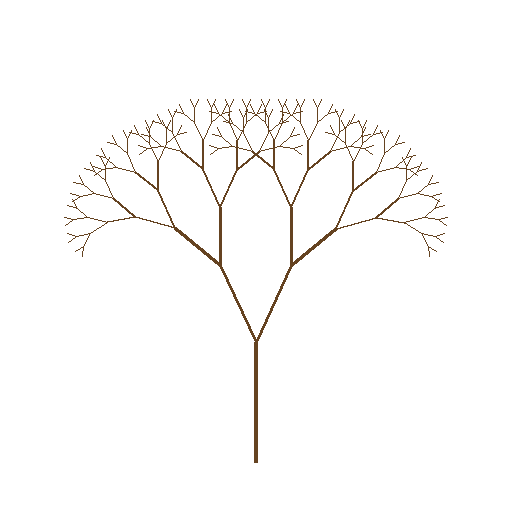

Core concepts

Concept 1 — Why trees are fractal

Self-similarity in real trees is not a metaphor — it is the visible signature of the recursive growth program in the plant’s apical meristem. At every growth event, the tip either elongates (extending the current branch) or branches (creating two new tips) [3]. The number, angle, and length ratios of these branchings are determined by genetics; the resulting shape is whatever satisfies three competing pressures:

• Maximise light capture — wider angles spread leaves into more sky.
• Minimise self-shading — branches that overlap waste their own canopy.
• Stay mechanically stable — too much weight on a long thin branch breaks it.

Hisao Honda’s classical 1971 model showed that just three parameters — branching angle, length ratio, and total depth — already produce silhouettes that match real species closely enough for botanical identification [4]. Pines have narrow angles, oaks have wide angles, willows have steep starting angles.

Concept 2 — The recursive algorithm

The recursion has the standard fractal anatomy: base case + recursive case.

def draw_branch(draw, x, y, length, angle, depth, branch_angle, length_ratio):
    # Base case
    if depth == 0:
        return

    # Compute endpoint with polar-to-Cartesian
    end_x = x + length * math.sin(angle)
    end_y = y - length * math.cos(angle)         # subtract: y grows downward

    # Draw this branch
    thickness = max(1, depth // 2)               # tapers with depth
    draw.line([(x, y), (end_x, end_y)],
              fill=(101, 67, 33), width=thickness)

    # Recursive case: two child branches
    new_length = length * length_ratio
    draw_branch(draw, end_x, end_y, new_length,
                angle - branch_angle, depth - 1, branch_angle, length_ratio)
    draw_branch(draw, end_x, end_y, new_length,
                angle + branch_angle, depth - 1, branch_angle, length_ratio)

Three things to notice. First, the angle is measured from vertical — angle = 0 points straight up. The trig formulas $\sin$/$\cos$ assume that convention. Second, end_y = y - length * cos(angle) because Pillow’s coordinate system has y growing downward; subtracting moves the endpoint up. Third, the thickness taper max(1, depth // 2) is purely cosmetic but doubles the visual realism — real branches taper, and so should yours.

Concept 3 — Three parameters, infinite trees

The three knobs:

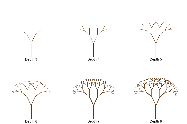
• Depth controls how many levels of branching occur. Each level doubles the branch count: depth $n$ produces “two to the n+1 minus one” branches. Past depth 12 the recursion limit and the runtime both become problems.
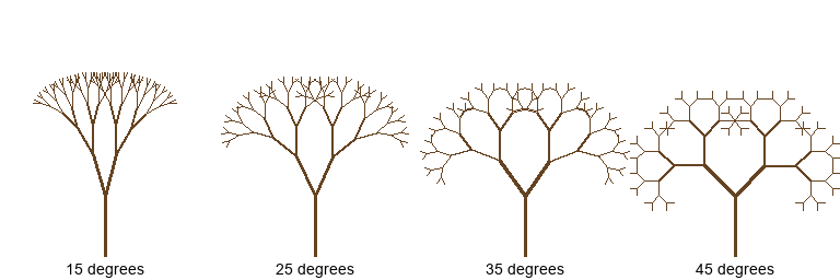
• Branch angle controls how wide the tree spreads. Small angles (10–15°) give pine-like silhouettes that lift toward the sky. Wide angles (40°+) give oak-like spreading canopies.
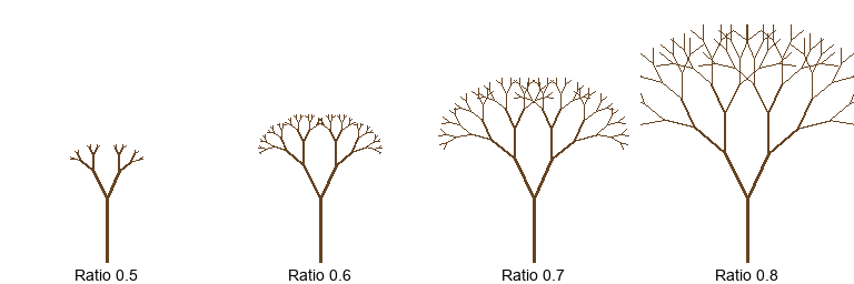
• Length ratio controls how quickly the branches shrink. Below 0.5 the tree is sparse and obviously fractal; above 0.8 the children almost equal their parent and the tree fills out into a dense ball.

Exercises

Three exercises in Execute → Modify → Create order: run the default tree, tune the three parameters, then add randomness to make it organic.

CREATE III.

Add organic randomness

Convert the deterministic tree into a stochastic one by jittering each recursion’s angle and length ratio. Start from the deterministic version in the starter, then complete the TODOs.

python · exercise3_starter.py Copy

import math
import random
from PIL import Image, ImageDraw

def draw_branch_organic(draw, x, y, length, angle, depth, branch_angle, length_ratio):
    if depth == 0 or length < 2:
        return

    # TODO 1: jitter the angle by uniform(-0.15, 0.15) radians (~ ±9°)

    # TODO 2: jitter the length ratio by uniform(-0.1, +0.1), clipped to [0.4, 0.9]

    # TODO 3: 10% chance to skip drawing this branch entirely (organic gaps)

    end_x = x + length * math.sin(angle)
    end_y = y - length * math.cos(angle)
    draw.line([(x, y), (end_x, end_y)], fill=(101, 67, 33), width=max(1, depth // 2))

    new_length = length * length_ratio
    draw_branch_organic(draw, end_x, end_y, new_length,
                        angle - branch_angle, depth - 1, branch_angle, length_ratio)
    draw_branch_organic(draw, end_x, end_y, new_length,
                        angle + branch_angle, depth - 1, branch_angle, length_ratio)

random.seed(0)
img = Image.new('RGB', (512, 512), 'white')
draw_branch_organic(ImageDraw.Draw(img), 256, 462, 120, 0, 9, math.radians(25), 0.72)
img.save('natural_tree.png')

fractal_tree_starter.py — deterministic skeleton

Hint 1 — jitter the angle

angle += random.uniform(-0.15, 0.15)

Insert this before computing end_x/end_y. Each branch picks its own random offset, so the perturbation is independent at every recursion level.

Hint 2 — jitter the length ratio

length_ratio = max(0.4, min(0.9, length_ratio + random.uniform(-0.1, 0.1)))

Clipping prevents both shrinkage too fast (branches vanish) and growth (children longer than parents → recursion explosion).

Hint 3 — random branch dropout

if random.random() < 0.1:
    return

Insert this before drawing. 10% of branches are skipped, producing the characteristic asymmetric gaps of real trees. Raise it to 0.3 for sparse winter trees.

Complete solution

python · exercise3_solution.py Copy

import math, random
from PIL import Image, ImageDraw

def draw_branch_organic(draw, x, y, length, angle, depth, branch_angle, length_ratio):
    if depth == 0 or length < 2:
        return
    if random.random() < 0.1:
        return

    angle += random.uniform(-0.15, 0.15)
    length_ratio = max(0.4, min(0.9, length_ratio + random.uniform(-0.1, 0.1)))

    end_x = x + length * math.sin(angle)
    end_y = y - length * math.cos(angle)
    draw.line([(x, y), (end_x, end_y)], fill=(101, 67, 33), width=max(1, depth // 2))

    new_length = length * length_ratio
    draw_branch_organic(draw, end_x, end_y, new_length,
                        angle - branch_angle, depth - 1, branch_angle, length_ratio)
    draw_branch_organic(draw, end_x, end_y, new_length,
                        angle + branch_angle, depth - 1, branch_angle, length_ratio)

random.seed(0)
img = Image.new('RGB', (512, 512), 'white')
draw_branch_organic(ImageDraw.Draw(img), 256, 462, 120, 0, 9, math.radians(25), 0.72)
img.save('natural_tree.png')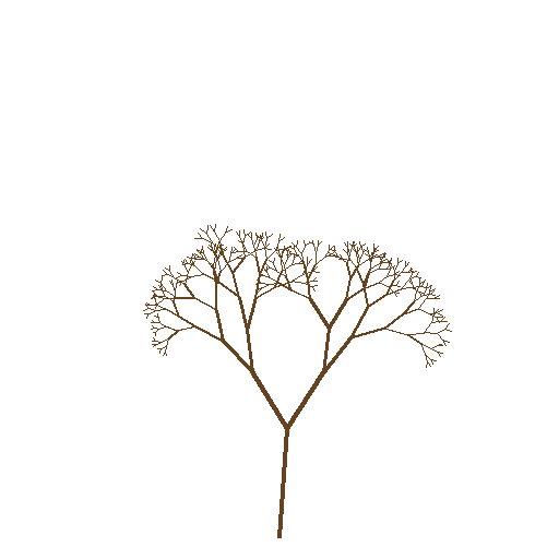

Make it your own

• Seasonal palette. Add green-leaf circles when depth <= 1. Mix red and yellow circles via random.random() for autumn.
• Wind. Multiply every branch’s angle by 1 + 0.1 * math.sin(time) — pass a single global time parameter through the recursion. Render frames at $t = 0, 0.1, 0.2, \ldots$ for an animated GIF.
• Forest. Run the tree 10 times at different start_x positions with different random seeds. Vary length_ratio and branch_angle per tree. Stack them at different starting y values for a depth-of-field forest.

Downloads

Summary

Common pitfalls to avoid

• Adding instead of subtracting cos(angle). Pillow’s y-axis points down. Subtract or your tree grows into the floor.
• Depth > 11 with the default Python recursion limit (1000). Two to the twelfth = 4,096 branch calls — manageable, but call stack depth grows linearly with the binary-tree depth. Raise sys.setrecursionlimit or refactor to an iterative version if you need very deep trees.
• Length ratio ≥ 1. Children grow longer than parents; recursion explodes. Keep length_ratio strictly below 1.
• Forgetting length < 2 short-circuit. With jitter, a child branch can become microscopically short and waste recursion levels. Bail out when sub-pixel.

References

- [1] Mandelbrot, B. B. (1982). The Fractal Geometry of Nature. W. H. Freeman. ISBN 978-0-7167-1186-5.
- [2] West, G. B., Brown, J. H., & Enquist, B. J. (1999). A general model for the structure and allometry of plant vascular systems. Nature, 400, 664–667. doi:10.1038/23251
- [3] Prusinkiewicz, P., & Lindenmayer, A. (1990). The Algorithmic Beauty of Plants. Springer-Verlag. ISBN 978-0-387-97297-8.
- [4] Honda, H. (1971). Description of the form of trees by the parameters of the tree-like body. Journal of Theoretical Biology, 31(2), 331–338. doi:10.1016/0022-5193(71)90191-3
- [5] Eloy, C. (2011). Leonardo’s rule, self-similarity, and wind-induced stresses in trees. Physical Review Letters, 107(25), 258101. doi:10.1103/PhysRevLett.107.258101
- [6] Barnsley, M. F. (1988). Fractals Everywhere. Academic Press. ISBN 978-0-12-079062-9.
- [7] Shiffman, D. (2012). The Nature of Code: Simulating Natural Systems with Processing. natureofcode.com.