1.2.1 Random Pattern Generation
Turn uniform random numbers into compelling visual compositions. Use Kronecker products for pixel-perfect scaling, seed-based reproducibility, and discrete colour palettes inspired by Gerhard Richter's colour charts.
Overview
Random number generation is a fundamental building block of computational art and generative design. In this lesson you will discover how simple random processes can create compelling visual patterns, from abstract colour compositions to structured artistic grids inspired by pioneers like Gerhard Richter [1].
Learning objectives
- Understand how uniform random distributions create unbiased colour sampling for image generation.
- Use Kronecker products to efficiently scale small pixel grids into pixel-perfect tile patterns.
- Recognise how colour space properties affect the visual perception of randomness.
- Create Richter-inspired discrete-palette compositions using index-based colour mapping.
Quick start — see randomness in action
Run this code to generate a random colour tile pattern:
import numpy as np
from PIL import Image

# Set seed for reproducible randomness
np.random.seed(42)

# Create 10x10 grid of random RGB colors
random_colors = np.random.randint(0, 256, size=(10, 10, 3), dtype=np.uint8)

# Scale each color to a 20x20 pixel tile using Kronecker product
scaled_image = np.kron(random_colors, np.ones((20, 20, 1), dtype=np.uint8))

# Save the result
result = Image.fromarray(scaled_image)
result.save('quick_random_tiles.png')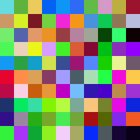
Core concepts
Concept 1 — Uniform random distribution
The uniform distribution is the foundation of digital randomness. When you call np.random.randint(0, 256), every integer from 0 to 255 has an equal probability of being selected [2]. This creates what we perceive as “pure randomness.”
import numpy as np

# Every RGB value has equal 1/256 probability
random_rgb = np.random.randint(0, 256, size=(5, 5, 3), dtype=np.uint8)

# This gives us 256^3 = 16,777,216 possible colors per pixel
total_colors = 256 ** 3
print(f"Total possible colors: {total_colors:,}")
For generative art, uniform distribution provides three key properties:
- Unpredictability — no discernible patterns in individual elements.
- Visual balance — all colours represented equally over large samples.
- Infinite variety — each generation produces unique results.
Concept 2 — Kronecker product for scaling
The Kronecker product (np.kron) is a linear algebra operation that efficiently scales images by repeating each pixel into a larger block [4]. Instead of writing nested loops, you get pixel-perfect tile scaling in a single function call.
import numpy as np

# Original: 2x2 array
small = np.array([[1, 2], [3, 4]])

# Scaling matrix: each element becomes a 3x3 block
scale = np.ones((3, 3))

# Kronecker product result: 6x6 array
large = np.kron(small, scale)
# Result: each original value repeated in 3x3 blocks
print(large)
For images, this transforms a small random grid into pixel-perfect tiles:
import numpy as np

# Small random grid: 5x5x3 (75 total color values)
small_grid = np.random.randint(0, 256, size=(5, 5, 3), dtype=np.uint8)

# Scale each color to a 40x40 pixel tile
tile_size = np.ones((40, 40, 1), dtype=np.uint8)
large_image = np.kron(small_grid, tile_size)
# Result: 200x200x3 image (40,000 pixels, but only 75 unique color values)
The third dimension of the scaling matrix is 1 rather than 3 because each colour channel scales independently. The Kronecker product broadcasts the single-channel scale across all three RGB channels.
Concept 3 — Colour space considerations
When generating random colours, the choice of colour space dramatically affects the visual result [5]:
- RGB space — uniform in red, green, and blue channels independently.
- Perceptual uniformity — RGB is not perceptually uniform. Some random colours appear much brighter than others.
- Gamut coverage — random RGB covers the entire digital colour palette, including colours that rarely appear in nature.
import numpy as np

# These are all equally "random" in RGB space
color1 = [255, 255, 255]  # Bright white
color2 = [128, 128, 128]  # Medium gray
color3 = [255, 0, 0]      # Pure red
color4 = [1, 1, 1]        # Nearly black

# But they have very different perceptual brightness!
This perceptual non-uniformity creates visually interesting compositions because the eye perceives some tiles as “popping forward” (bright colours) while others recede (dark colours), adding implicit depth to a flat, two-dimensional pattern.
Exercises
Three progressively challenging exercises, each building on the previous using the Execute → Modify → Create approach.
Random colour tiles
Run the following code exactly as written and observe the output. This creates a grid of random coloured tiles using uniform distribution and Kronecker scaling.
import numpy as np
from PIL import Image

# Create a 10x10 grid of random RGB colors
random_colors = np.random.randint(0, 256, size=(10, 10, 3), dtype=np.uint8)

# Scale each color to a 20x20 pixel tile using Kronecker product
scaling_matrix = np.ones((20, 20, 1), dtype=np.uint8)
image_array = np.kron(random_colors, scaling_matrix)

# Convert to image and save
result_image = Image.fromarray(image_array)
result_image.save('random_tiles.png')

print(f"Image dimensions: {image_array.shape}")
Reflection questions
- What do you notice about the colours? Are any two tiles exactly the same?
- Why does each tile appear as a solid block rather than individual pixels?
- What role does the Kronecker product play in creating the final image?
Solution & explanation
What happened:
np.random.randint(0, 256, ...)creates a 10x10x3 array where each RGB value is randomly chosen from 0—255.np.kron()scales each colour into a 20x20 pixel block, creating the tile effect.- The final image is 200x200 pixels (10 tiles x 20 pixels per tile).
Key insights:
- Each tile is a different random colour due to uniform distribution.
- The Kronecker product efficiently repeats each colour value into larger blocks — no loops needed.
- You get 100 unique colours (10x10 tiles) drawn from 16.7 million possible RGB combinations. The chance of two tiles being identical is astronomically small.
Tune the parameters
Open exercise1_execute.py from Exercise 1 and modify the marked parameters to achieve each of these different effects. Change only the specified values, then re-run.
Goals
- Muted palette — change the colour range to produce soft, pastel-like tones only.
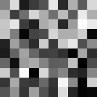
- Grayscale tiles — make all tiles appear in shades of gray.
- Larger, bolder tiles — increase the tile size for a more graphic effect.
Goal 1 — what to expect
Limit the random range to a narrow band of middle values. Instead of spanning 0—255, try generating values between 100 and 180. The result is a composition of soft, muted colours — no harsh blacks, no blinding whites. The palette feels cohesive even though each tile is still random.
Goal 2 — what to expect
When all three RGB channels share the same value, the result is a shade of gray. Generate a single-channel random grid and stack it across all three channels. The composition shifts from a colourful mosaic to a study in light and shadow.
Goal 3 — what to expect
Increasing the scaling matrix from (20, 20, 1) to (40, 40, 1) doubles each tile’s size. The image grows from 200x200 to 400x400 pixels, and the composition reads as a bolder, more graphic pattern — fewer tiles visible at once, each commanding more visual weight.
Hints
- For muted colours: change the range in
np.random.randint(100, 180, ...). - For grayscale: generate a 2D array and use
np.stackto repeat it across three channels. - For larger tiles: increase the scaling matrix dimensions.
Solutions
1. Muted palette:
# Change this line:
random_colors = np.random.randint(100, 180, size=(10, 10, 3), dtype=np.uint8)
# Creates colors only in the 100-179 range (muted/pastel effect)
2. Grayscale tiles:
# Generate grayscale values and repeat across RGB channels
gray_values = np.random.randint(0, 256, size=(10, 10), dtype=np.uint8)
random_colors = np.stack([gray_values, gray_values, gray_values], axis=2)
3. Larger tiles:
# Change this line:
scaling_matrix = np.ones((40, 40, 1), dtype=np.uint8)
# Creates 40x40 pixel tiles instead of 20x20Richter-inspired discrete palette
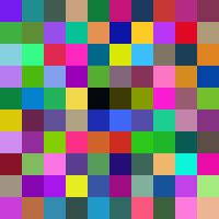
Create something new: a colour grid inspired by Gerhard Richter’s 1024 Colours (1973) [1] using only discrete colour values. Instead of the full 0—255 range, restrict each channel to eight specific values — producing a structured, limited-palette composition.
Goal: Create random tiles that use only colour values divisible by 32 (0, 32, 64, 96, 128, 160, 192, 224) on a 16x16 grid with 12x12 pixel tiles.
import numpy as np
from PIL import Image

# Discrete color palette (values divisible by 32)
color_palette = np.array([0, 32, 64, 96, 128, 160, 192, 224])

# TODO 1: Create a 16x16 grid of random indices into the palette
#         (each index selects one of the 8 palette values, for each of 3 channels)

# TODO 2: Map the random indices to actual color values using array indexing

# TODO 3: Scale up to 12x12 pixel tiles using the Kronecker product and save as
#         'richter_style.png'
Hint 1 — generating palette indices
Use np.random.randint(0, len(color_palette), size=(16, 16, 3)) to pick a random index for each channel of each tile. The indices range from 0 to 7, corresponding to the eight palette values.
Hint 2 — mapping indices to colour values
NumPy’s advanced indexing lets you use an array of indices to look up values in another array: color_palette[random_indices]. This converts every index into its corresponding palette value in one vectorised step.
Hint 3 — Kronecker scaling
The same pattern from the earlier exercises applies: create a scaling matrix with np.ones((12, 12, 1), dtype=np.uint8) and pass it to np.kron alongside the colour grid. Remember to cast the colour grid to uint8 before scaling.
Complete solution
import numpy as np
from PIL import Image

# Discrete color palette (values divisible by 32)
color_palette = np.array([0, 32, 64, 96, 128, 160, 192, 224])

# Generate random indices into the palette for a 16x16 grid
random_indices = np.random.randint(0, len(color_palette), size=(16, 16, 3))

# Map indices to actual color values
small_array = color_palette[random_indices].astype(np.uint8)

# Scale each color to 12x12 pixel tiles
scaling_matrix = np.ones((12, 12, 1), dtype=np.uint8)
image_array = np.kron(small_array, scaling_matrix)

# Save result
result_image = Image.fromarray(image_array)
result_image.save('richter_style.png')
print(f"Created {image_array.shape} Richter-style grid!")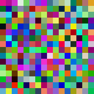
How it works:
np.random.randint(0, len(color_palette), size=(16, 16, 3))creates a grid of indices (0—7) for each RGB channel of each tile.color_palette[random_indices]maps those indices to actual colour values using NumPy’s advanced indexing.- The result uses only 8 values per channel, giving 8 x 8 x 8 = 512 possible colours instead of 16.7 million. This constrained palette produces the structured, harmonious aesthetic characteristic of Richter’s colour charts [1].
Make it your own
After the TODOs work, try these extensions by editing the script directly:
- Change the palette to fewer values (e.g.
[0, 85, 170, 255]— four values per channel, 64 total colours). - Try a warm-only palette: restrict the red channel to high values and the blue channel to low values.
- Increase the grid to 32x32 tiles with 6x6 pixel size for a denser, more textile-like composition.
- Add a seed with
np.random.seed(...)and find a composition you like. Record the seed number so you can reproduce it later.
Downloads
random_tiles.py — combined scriptSummary
Common pitfalls to avoid
- Forgetting
dtype=np.uint8— Pillow expects unsigned 8-bit integers for standard images. Without this,Image.fromarraymay produce unexpected results or errors. - Confusing the Kronecker scaling matrix shape — the third dimension should be
1(not3) so broadcasting works correctly across all three RGB channels. - Running without a seed and expecting the same output — each run produces a different image unless you set
np.random.seed()beforehand. - Using
np.random.rand()(float 0—1) instead ofnp.random.randint()(integer 0—255) for direct image arrays. Float arrays require multiplication and casting before they work with Pillow.
References
- [1] Richter, G. (1973). 1024 Colours [Oil on canvas, No. 350]. Gerhard Richter Archive. gerhard-richter.com
- [2] Knuth, D. E. (1997). The Art of Computer Programming, Volume 2: Seminumerical Algorithms (3rd ed.). Addison-Wesley.
- [3] NumPy Community. (2023). Random sampling (numpy.random). NumPy Documentation, version 1.24. numpy.org
- [4] Horn, R. A., & Johnson, C. R. (2012). Matrix Analysis (2nd ed.). Cambridge University Press.
- [5] Fairchild, M. D. (2013). Color Appearance Models (3rd ed.). Wiley. ISBN 978-1-119-96703-3.
- [6] Harris, C. R., et al. (2020). Array programming with NumPy. Nature, 585, 357–362. doi:10.1038/s41586-020-2649-2
- [7] Galanter, P. (2003). What is generative art? Complexity theory as a context for art theory. In Proceedings of the 6th Generative Art Conference. Politecnico di Milano.