1.2.2 Cellular Automata (Game of Life)

Overview

Five live cells on a 20×20 grid. Eight frames later, those five cells have walked diagonally across the canvas — without a single line of movement code. That illusion of motion comes from one of the most studied systems in twentieth-century mathematics: Conway’s Game of Life [1]. Four arithmetic rules, applied uniformly to every cell, produce structures that move, blink, and persist [2].

Learning objectives

1. Implement Conway’s Game of Life as a synchronous update over a 2D NumPy grid.
2. Count Moore-neighbourhood neighbours in parallel using a SciPy 2D convolution.
3. Recognise the three pattern classes — still lifes, oscillators, spaceships — by their neighbour-count signatures.
4. Reason about how boundary conditions (toroidal vs fixed) reshape a pattern’s evolution.

Quick start — see life in action

import numpy as np
from PIL import Image
from scipy.ndimage import convolve
import imageio

def grid_to_image(grid, scale=8):
    """Convert binary grid to grayscale image."""
    return np.repeat(np.repeat(grid * 255, scale, axis=0), scale, axis=1).astype(np.uint8)

grid = np.zeros((20, 20), dtype=int)
grid[8:11, 8:11] = [[0, 1, 0], [0, 0, 1], [1, 1, 1]]  # Glider

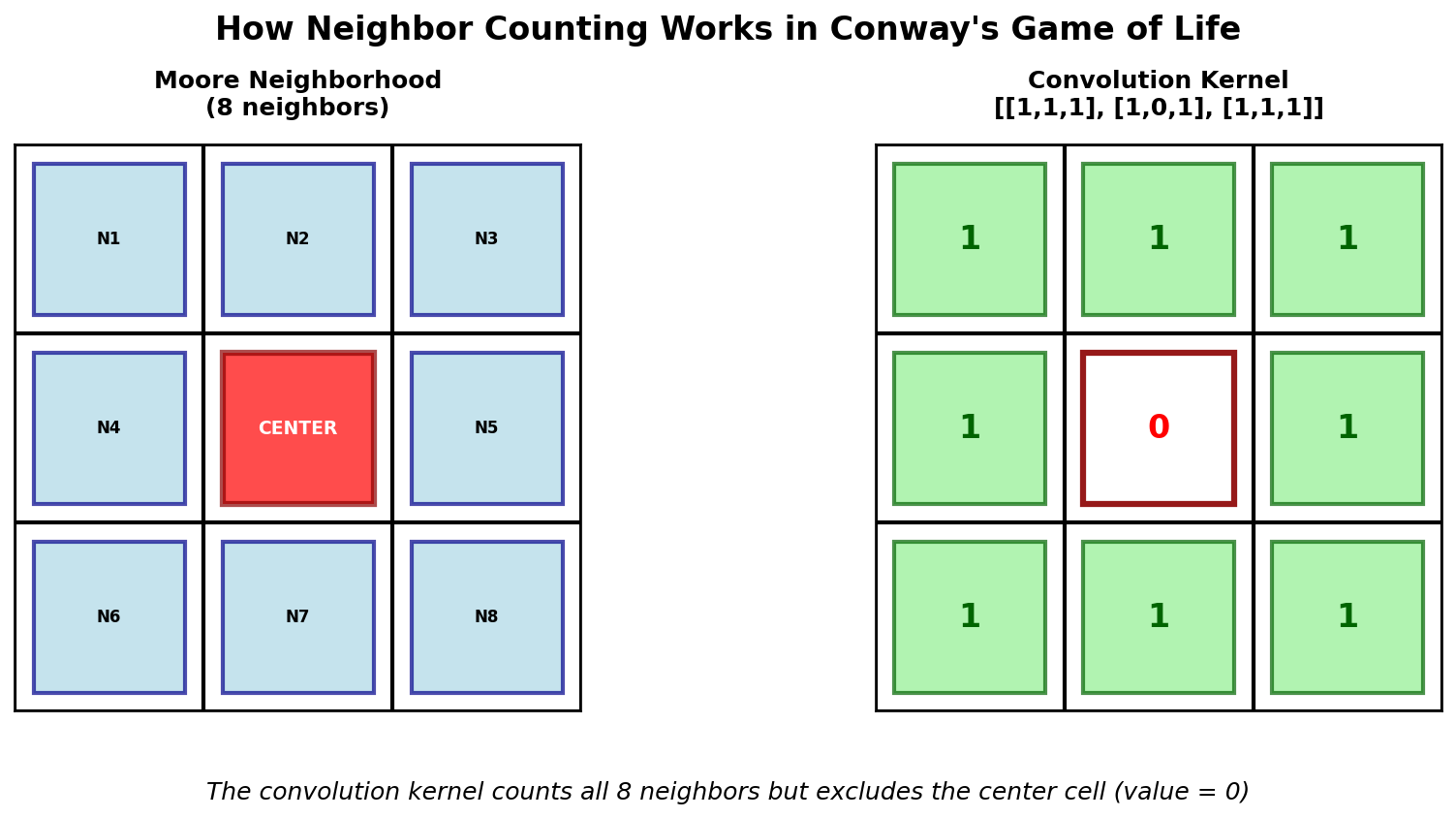
# Moore neighbourhood kernel (counts 8 surrounding cells, excludes centre)
kernel = np.array([[1, 1, 1],
                   [1, 0, 1],
                   [1, 1, 1]])

frames = []
for step in range(8):
    frames.append(grid_to_image(grid))
    neighbor_count = convolve(grid, kernel, mode='wrap')
    # Apply B3/S23 rules
    birth = (neighbor_count == 3)
    survival = (grid == 1) & (neighbor_count == 2)
    grid = (birth | survival).astype(int)

imageio.mimsave('glider_animation.gif', frames, fps=2, duration=0.5)

Core concepts

Concept 1 — What a cellular automaton is

A cellular automaton is three things plus one constraint [2]:

1. A grid — a regular array of cells, each in one of a small set of states (here: alive 1 or dead 0).
2. A rule — a function that determines a cell’s next state from its current state and the states of its neighbours.
3. Discrete time — every cell updates at once on each tick.

grid = np.zeros((height, width), dtype=int)   # 0 = dead, 1 = alive

for generation in range(num_steps):
    grid = apply_rules(grid)                   # all cells update together

This framework, despite its plainness, generates four qualitatively distinct long-run dynamics [2]: static equilibria, periodic cycles, traveling structures, and unbounded chaotic transients. Conway’s rules sit in the corner of rule space where all four can coexist on the same grid.

Conway’s rules (B3/S23)

The Game of Life uses four rules over each cell’s eight neighbours — the Moore neighbourhood [1]:

• Birth — a dead cell with exactly 3 living neighbours becomes alive.
• Survival — a living cell with 2 or 3 living neighbours stays alive.
• Death by isolation — a living cell with fewer than 2 neighbours dies.
• Death by overcrowding — a living cell with more than 3 neighbours dies.

birth     = (neighbor_count == 3) & (grid == 0)
survival  = (neighbor_count >= 2) & (neighbor_count <= 3) & (grid == 1)
new_grid  = (birth | survival).astype(int)

These rules sort almost any starting pattern into three pattern categories [3]: still lifes (unchanging), oscillators (periodic), and spaceships (traveling).

Concept 2 — Pattern classification

Each pattern category has a recognisable signature once you know what to look for [3].

Still lifes — stable forever. The smallest is the block [9]: a 2×2 square where every living cell has exactly three living neighbours (counted including diagonals) and every adjacent dead cell has fewer than three. Nothing is born, nothing dies — perfect stability.

Generation 0:    Generation 1:    Generation 2:
. . . .          . . . .          . . . .
. ■ ■ .    →     . ■ ■ .    →     . ■ ■ .
. ■ ■ .          . ■ ■ .          . ■ ■ .
. . . .          . . . .          . . . .

Oscillators — rhythmic patterns. The blinker alternates between horizontal and vertical orientations every generation:

Generation 0:    Generation 1:    Generation 2:
. . . . .        . . ■ . .        . . . . .
. ■ ■ ■ .   →    . . ■ . .   →    . ■ ■ ■ .
. . . . .        . . ■ . .        . . . . .

The horizontal line becomes vertical, then horizontal again. This is a period-2 oscillator [9].

A more theatrical oscillator is the beacon, which alternates between six and eight living cells:

Generation 0:    Generation 1:    Generation 2:
■ ■ . .          ■ ■ . .          ■ ■ . .
■ . . .    →     ■ ■ . .    →     ■ . . .
. . . ■          . . ■ ■          . . . ■
. . ■ ■          . . ■ ■          . . ■ ■

Spaceships — moving patterns. Where an oscillator transforms in place, a spaceship rebuilds itself one cell over each cycle. The glider moves diagonally:

Step 0:          Step 1:          Step 2:          Step 4:
. ■ . . .        . . . . .        . . . . .        . . . . .
. . ■ . .   →    ■ . ■ . .   →    . . ■ . .   →    . . . ■ .
■ ■ ■ . .        . ■ ■ . .        ■ . ■ . .        . . ■ ■ .
. . . . .        . ■ . . .        . ■ ■ . .        . . ■ . .

The glider reconstructs itself one cell down and one cell to the right every four generations [1] — the illusion of motion produced entirely by arithmetic.

Placing patterns in code

Every Game of Life pattern is a small 2D shape that you drop onto the grid via array slicing. Read the visual row by row, converting filled cells to 1 and empty cells to 0:

# Horizontal blinker (1 row × 3 columns):
# ■ ■ ■
grid[10, 5:8] = [1, 1, 1]

# Vertical blinker (3 rows × 1 column):
# ■
# ■
# ■
grid[10:13, 5] = [1, 1, 1]

# Glider (3 rows × 3 columns) — read row by row:
# . ■ .     →  [0, 1, 0]
# . . ■     →  [0, 0, 1]
# ■ ■ ■     →  [1, 1, 1]
grid[10:13, 5:8] = [[0, 1, 0], [0, 0, 1], [1, 1, 1]]

To rotate a pattern, rearrange the rows. A glider heading up-left instead of down-right:

# Glider rotated 180°:
# ■ ■ ■     →  [1, 1, 1]
# ■ . .     →  [1, 0, 0]
# . ■ .     →  [0, 1, 0]
grid[10:13, 5:8] = [[1, 1, 1], [1, 0, 0], [0, 1, 0]]

Concept 3 — Neighbour counting via convolution

The standard, blazingly fast approach to neighbour counting is a 2D convolution [8] with a kernel shaped like the Moore neighbourhood:

# Counts each cell's 8 neighbours (centre 0 excludes the cell itself)
kernel = np.array([[1, 1, 1],
                   [1, 0, 1],
                   [1, 1, 1]])

neighbor_count = convolve(grid, kernel, mode='wrap')

Convolution counts every cell’s neighbours in parallel, so the algorithm scales to large grids without nested Python loops. mode='wrap' produces toroidal boundary conditions [2] — opposite edges of the grid are connected.

Concept 4 — Boundary conditions reshape evolution

How the grid handles its edges changes pattern behaviour at the boundary [6]:

• Wrap-around (torus) — mode='wrap', patterns can move continuously across the edge.
• Fixed dead boundary — mode='constant', cells beyond the edge act as permanently dead — a wall.
• Reflective — custom implementation, patterns bounce off the edge.

wrap_neighbors  = convolve(grid, kernel, mode='wrap')     # toroidal
fixed_neighbors = convolve(grid, kernel, mode='constant') # dead boundary

For art and exploration, wrap-around produces more interesting long-run behaviour [6] because patterns can interact across the entire space. For studying single patterns in isolation, a fixed boundary acts like a black hole at the edge.

Exercises

Three exercises in the standard Execute → Modify → Create progression [10, 11].

EXECUTE I.

The blinker

The blinker is the simplest oscillator — three cells, period 2. Run it and watch the line flip.

bash Copy

python exercise1_execute.py

Reflection questions

• Does the living-cell count change, or does it stay at exactly 3?
• Can you trace, in your head, how the horizontal line becomes vertical, then horizontal again?
• Which pattern category (still life / oscillator / spaceship) does the blinker belong to, and why?

Solution & explanation

The blinker maintains exactly three living cells throughout. Odd generations show a vertical line (three cells in a column); even generations show a horizontal line (three cells in a row). The pattern returns to its starting state every two ticks — a period-2 oscillator.

Why exactly three cells? The end cells each have only one living neighbour, so they die. The middle cell has two living neighbours, so it survives. Two new cells are born above and below the middle (each has exactly three living neighbours). Net: three cells, rotated 90°.

MODIFY II.

Blinker variations

Open exercise2_modify.py. The script starts with a blinker at the centre of a 30×30 grid. Change the marked values to hit each goal below, then re-run.

bash Copy

python exercise2_modify.py

Goals

1. Move the blinker to the very top edge — change its position to row 0. Does it still oscillate?
2. Switch boundary mode — keep the edge blinker and change mode='wrap' to mode='constant'. What happens?
3. Multiple blinkers — add several blinkers at different positions and orientations.

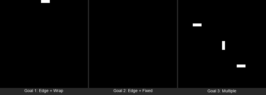
Goal 1 — what to expect

Change the placement line to grid[0, 14:17] = [1, 1, 1]. With wrap-around boundaries, the blinker oscillates normally even at the top edge because the grid is a torus — cells “above” row 0 wrap around to the bottom rows. The blinker survives.

Goal 2 — what to expect

Inside game_of_life_step, change the convolution to mode='constant'. Combined with the edge placement from goal 1, cells beyond the edge are now treated as permanently dead. The blinker loses the neighbours it needs to survive and dies within two generations — the grid goes empty. Boundary conditions can be the difference between life and death.

Goal 3 — what to expect

Each blinker oscillates independently as long as they are far enough apart. Mixing horizontal and vertical blinkers shows both orientations alive at once.

Experiment: place two horizontal blinkers two rows apart (e.g. rows 14 and 16) and watch their interaction.

Solutions

python Copy

# 1. Edge blinker
grid[0, 14:17] = [1, 1, 1]

# 2. Fixed boundaries — in game_of_life_step:
neighbor_count = convolve(grid, kernel, mode='constant')

# 3. Multiple blinkers
grid[8, 5:8]    = [1, 1, 1]   # horizontal
grid[14:17, 15] = [1, 1, 1]   # vertical
grid[22, 20:23] = [1, 1, 1]   # horizontal

CREATE III.

A pattern garden

Open exercise3_create.py. The helper functions and grid setup are provided. Complete the three TODOs to place an oscillator and a spaceship on the same grid and let them coexist for twenty generations.

bash Copy

python exercise3_create.py

Hint 1 — review the pattern shapes

The beacon’s bottom-right block mirrors the top-left block:

• Top-left: [[1, 1], [1, 0]] — full top row, left cell on the bottom.
• Bottom-right: think of it as the opposite. What fills the bottom row and the right cell on top?

For the glider, read the visual row by row, converting filled squares to 1 and empty to 0.

Hint 2 — 2D slice indexing

A 2D list like [[0, 1], [1, 1]] assigns row-by-row into a grid slice. grid[7:9, 7:9] means rows 7 and 8, columns 7 and 8 — a 2×2 region. grid[20:23, 10:13] means rows 20–22, columns 10–12 — a 3×3 region.

Hint 3 — partial code

python Copy

# TODO 1 — beacon's bottom-right block:
grid[7:9, 7:9] = [[0, 1], [1, 1]]

# TODO 2 — glider (first row given, complete the rest):
grid[20:23, 10:13] = [[0, 1, 0], ...]  # what are rows 2 and 3?

# TODO 3 — the evolution loop:
for generation in range(20):
    grid = game_of_life_step(grid)
    print(...)  # print generation number and np.sum(grid)

Complete solution

python · exercise3_solution.py Copy

# TODO 1 — beacon
grid[5:7, 5:7] = [[1, 1], [1, 0]]    # top-left block (provided)
grid[7:9, 7:9] = [[0, 1], [1, 1]]    # bottom-right block

# TODO 2 — glider
grid[20:23, 10:13] = [[0, 1, 0], [0, 0, 1], [1, 1, 1]]

# TODO 3 — evolution
for generation in range(20):
    grid = game_of_life_step(grid)
    print(f"Generation {generation + 1}: {np.sum(grid)} living cells")

How it works. The beacon oscillates between 6 and 8 cells but stays at its corner of the grid. The glider moves diagonally — five cells in twenty generations, exactly four ticks per cell. The two patterns coexist because they are far enough apart that their neighbour counts never overlap. Different pattern kinds on the same grid.

Make it your own

After the TODOs work, try these by editing the script directly:

• Add a single blinker: grid[row, col:col+3] = [1, 1, 1].
• Add a block (still life): grid[row:row+2, col:col+2] = 1.
• Place two gliders on a collision course. What happens when they meet?
• Push the grid to 60×60 and scatter many patterns. Density changes the dynamics.

Challenge — glider collision

python Copy

# Glider moving down-right
grid[5:8, 5:8] = [[0, 1, 0], [0, 0, 1], [1, 1, 1]]

# Glider moving up-left (rotated 180°)
grid[30:33, 30:33] = [[1, 1, 1], [1, 0, 0], [0, 1, 0]]

Run for 50+ generations and watch the collision. The outcome depends on exactly when and where the gliders meet. Sometimes they annihilate cleanly; sometimes they spawn debris that becomes new stable patterns.

Downloads

Summary

Common pitfalls to avoid

• Updating cells during the sweep instead of after. The grid must be read entirely from the current generation before any cell flips. Use a separate new_grid or NumPy’s convolve (which is implicitly synchronous).
• Forgetting mode='wrap' and then wondering why edge patterns die.
• Confusing the kernel with the rule — the kernel of ones only counts neighbours, it does not encode B3/S23. The rule lives in the birth/survival comparison afterwards.

References

- [1] Gardner, M. (1970). Mathematical Games: The fantastic combinations of John Conway’s new solitaire game “life”. Scientific American, 223(4), 120–123.
- [2] Wolfram, S. (2002). A New Kind of Science. Wolfram Media. ISBN 978-1-57955-008-0.
- [3] Adamatzky, A. (Ed.). (2010). Game of Life Cellular Automata. Springer. doi:10.1007/978-1-84996-217-9
- [4] Berlekamp, E. R., Conway, J. H., & Guy, R. K. (2004). Winning Ways for Your Mathematical Plays (2nd ed., Vol. 4, ch. 25). A K Peters.
- [5] Roberts, S. (2015). Genius at Play: The Curious Mind of John Horton Conway (pp. 125–126). Bloomsbury.
- [6] Flake, G. W. (1998). The Computational Beauty of Nature. MIT Press. ISBN 978-0-262-56127-3.
- [7] Von Neumann, J. (1966). Theory of Self-Reproducing Automata (A. W. Burks, Ed.). University of Illinois Press.
- [8] SciPy developers. (2024). scipy.ndimage.convolve. SciPy v1.12 Documentation. scipy.org
- [9] ConwayLife.com. (2024). LifeWiki: The wiki for Conway’s Game of Life. conwaylife.com
- [10] Sweller, J. (1988). Cognitive load during problem solving: Effects on learning. Cognitive Science, 12(2), 257–285. doi:10.1207/s15516709cog1202_4
- [11] Mayer, R. E. (2020). Multimedia Learning (3rd ed.). Cambridge University Press. ISBN 978-1-316-63816-1.