1.3.2 Repeat (Tiling Patterns)

Overview

Tiling patterns are the bridge between manual array slicing and procedural generation. In Module 1.3.1, you learned to select and modify rectangular regions using hardcoded slice positions like [0:150]. Now you will use nested loops to algorithmically calculate positions and create repeating grid patterns — the foundation of generative art.

This lesson introduces the concept of parametric variation: using formulas to create systematic changes across repeated elements. You will discover how a simple loop with a colour formula can generate gradients, checkerboards, and infinitely varying patterns.

Learning objectives

1. Use nested loops to iterate through 2D grid positions.
2. Calculate array slice positions algorithmically using formulas.
3. Create parametric colour variations based on position coordinates.
4. Understand the relationship between loop variables and pixel positions.

Quick start — create a tiling pattern

Run this script to create a 4x4 grid of coloured tiles. Each tile receives a different colour based on its position, producing a gradient effect:

import numpy as np
from PIL import Image

# Configuration parameters
N_TILES = 4          # Number of tiles per row/column
TILE_WIDTH = 125     # Width of each tile in pixels
SPACING = 15         # Gap between tiles
SIZE = TILE_WIDTH * N_TILES + SPACING

# Create blank canvas
canvas = np.zeros((SIZE, SIZE, 3), dtype=np.uint8)

# Nested loops to place tiles
for y in range(N_TILES):
    for x in range(N_TILES):
        # Calculate color based on position
        color = (50 * y + 50, 50 * x + 50, 0)

        # Calculate slice positions algorithmically
        row_start = SPACING + y * TILE_WIDTH
        row_stop = (y + 1) * TILE_WIDTH
        col_start = SPACING + x * TILE_WIDTH
        col_stop = (x + 1) * TILE_WIDTH

        # Place tile
        canvas[row_start:row_stop, col_start:col_stop] = color

# Save result
result = Image.fromarray(canvas, mode='RGB')
result.save('repeat.png')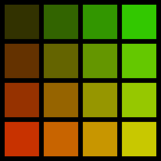

What you just created: a systematic pattern where each tile’s colour is determined by its position. The formula color = (50 * y + 50, 50 * x + 50, 0) creates a gradient: red values increase as you move down (higher y), and green values increase as you move right (higher x). This is parametric variation — using mathematical formulas to generate visual patterns.

Core concepts

Concept 1 — Algorithmic position calculation

In Module 1.3.1, you wrote slice positions manually: flag[:, 0:150] for a specific column range. But what if you need to place 10, 50, or 100 rectangles? Writing each position by hand becomes impractical.

The solution: use a formula to calculate positions based on a loop variable.

The general formula for positioning tiles in a grid is:

start = spacing + (i * tile_width)
stop = start + tile_width

Where i is the loop variable (0, 1, 2, 3, …). This formula ensures:

• Even spacing: each tile starts at a consistent offset from the previous one.
• Correct positioning: the spacing parameter creates gaps between tiles.
• Scalability: works for any number of tiles — just change the loop range.

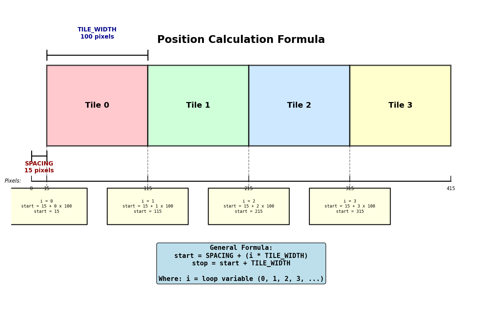
Example calculation for the second tile (i=1):

SPACING = 15
TILE_WIDTH = 125
i = 1

start = 15 + (1 * 125)  # = 140
stop = 140 + 125         # = 265

# Therefore: canvas[:, 140:265] selects the second tile's column range

This transforms static, manual slicing into dynamic, algorithmic positioning (Code.org, 2024). The same pattern extends to Truchet tiles, fractals, and procedural texture generation.

Concept 2 — Nested loops for 2D grid iteration

A nested loop is a loop inside another loop. For 2D grids, the outer loop controls rows (y-axis) and the inner loop controls columns (x-axis).

Basic structure:

for y in range(N_TILES):      # Outer loop: rows
    for x in range(N_TILES):  # Inner loop: columns
        # Process tile at position (x, y)

Execution order: the inner loop completes all its iterations before the outer loop advances. For a 4x4 grid:

1. Outer loop sets y=0.
2. Inner loop runs x=0, 1, 2, 3 (tiles 0—3).
3. Outer loop advances to y=1.
4. Inner loop runs x=0, 1, 2, 3 (tiles 4—7).
5. This continues until all 16 tiles are placed.

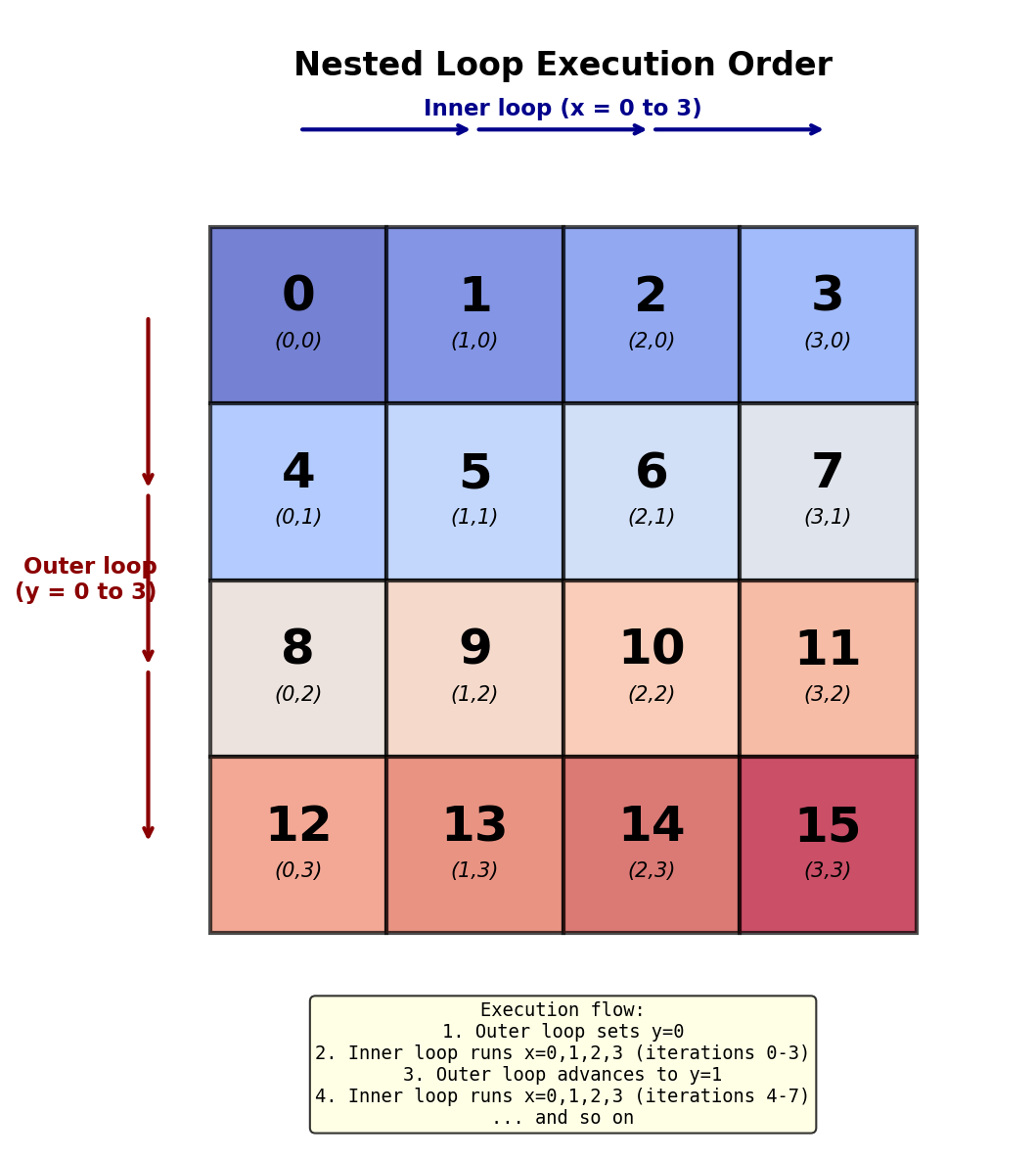
This execution pattern is critical for understanding how loops traverse 2D structures (OpenStax, 2024). Students often confuse the order, expecting tiles to be processed diagonally or in some other pattern. Visualising the iteration sequence demystifies nested loops and builds intuition for more complex algorithms.

Concept 3 — Parametric variation within patterns

Parametric variation means using formulas to create systematic changes across elements. Instead of manually assigning colours, you calculate them based on position:

color = (50 * y + 50, 50 * x + 50, 0)

This formula creates:

• Red channel: increases from 50 to 200 as y goes from 0 to 3.
• Green channel: increases from 50 to 200 as x goes from 0 to 3.
• Blue channel: constant at 0.

The result is a two-dimensional gradient (Galanter, 2016). By changing the formula, you create entirely different patterns:

Checkerboard alternation:

if (x + y) % 2 == 0:
    color = [0, 0, 0]        # Black
else:
    color = [83, 168, 139]   # Green

Diagonal gradient:

color = (0, 0, 30 * (x + y) + 50)  # Blue increases diagonally

Random variation:

color = (np.random.randint(0, 256),
         np.random.randint(0, 256),
         np.random.randint(0, 256))

The concept of algorithms + parameters = infinite variations is the essence of generative art (Pearson, 2011). The same loop structure creates vastly different outputs by changing the colour formula. This principle extends to texture synthesis, terrain generation, and procedural content in games.

Exercises

Three progressively challenging exercises, each building on the previous using the Execute, Modify, Create approach.

MODIFY II.

Explore tiling parameters

Modify the tiling pattern code to create different visual effects. Complete all three tasks.

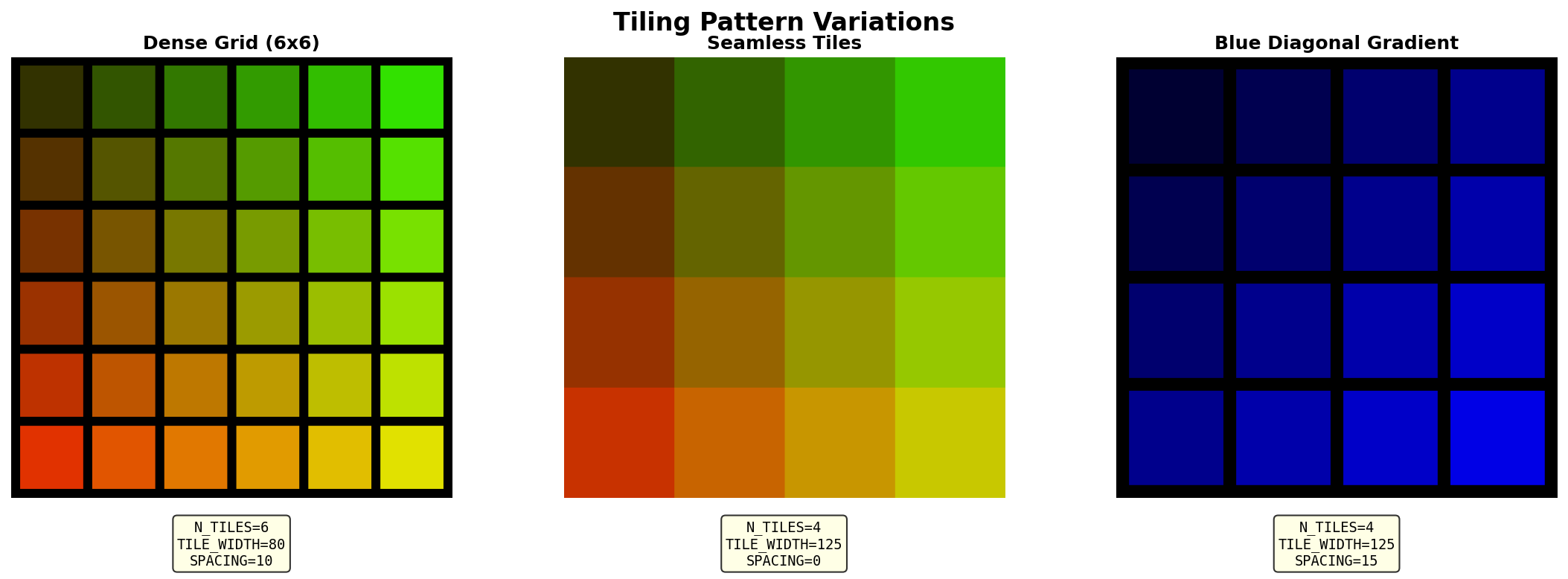
Goal 1 — Create a denser grid

Change N_TILES to 6 to create a 6x6 grid. Adjust TILE_WIDTH to fit the tiles in a 512x512 canvas.

What to expect

You should see 36 tiles instead of 16, each smaller than before, with a finer-grained colour gradient across the grid.

Hint: canvas size calculation

If you want a 512x512 canvas with 6 tiles and spacing, calculate:

python Copy

TILE_WIDTH = (512 - SPACING) // N_TILES
# For SPACING=15 and N_TILES=6: (512 - 15) // 6 = 82 pixels

Goal 2 — Experiment with spacing

Try these spacing values and observe how they affect the pattern:

• SPACING = 0 (seamless, tiles touch)
• SPACING = 30 (wide gaps between tiles)
• SPACING = 5 (narrow gaps)

What to expect

• SPACING = 0: creates a continuous gradient with no visual separation between tiles.
• SPACING = 30: creates prominent black gaps, emphasising individual tiles as distinct elements.
• SPACING = 5: subtle separation, balancing continuity with tile definition.

Goal 3 — Create a blue gradient

Modify the colour formula to create a diagonal blue gradient. Replace the existing formula with one that increases blue intensity diagonally from top-left to bottom-right.

Hint: diagonal direction

Use (x + y) to increase diagonally from top-left to bottom-right:

python Copy

color = (0, 0, min(255, 30 * (x + y) + 50))

The min(255, ...) ensures the value never exceeds 255.

Solutions

Goal 1 — Dense 6x6 grid

python Copy

N_TILES = 6
TILE_WIDTH = (512 - SPACING) // N_TILES  # 82 pixels for SPACING=15
SIZE = TILE_WIDTH * N_TILES + SPACING

This creates more tiles in the same canvas size, producing a denser pattern.

Goal 2 — Spacing effects

Each value changes the visual character of the grid without altering the colour logic. The spacing parameter controls whether the composition reads as a unified gradient or a collection of individual elements.

Goal 3 — Blue diagonal gradient

python Copy

color = (0, 0, min(255, 30 * (x + y) + 50))

This produces a gradient from dark blue (top-left, x+y=0) to bright blue (bottom-right, x+y=6).

CREATE III.

Build a checkerboard from scratch

Create a classic 8x8 checkerboard pattern with alternating black and green squares. This exercise tests your understanding of nested loops, position calculation, and alternation logic.

Requirements:

• 8x8 grid (standard chess/checkers board).
• No spacing between tiles (seamless).
• 64x64 pixel tiles (creates 512x512 canvas).
• Alternating black [0,0,0] and green [83,168,139] squares.

python · checkerboard_starter.py Copy

import numpy as np
from PIL import Image

# TODO 1: Define parameters
# What: set grid dimensions for an 8x8 board with 64px tiles
# Why: the tile size must divide evenly into 512 for seamless coverage
N_TILES = 8
TILE_SIZE = 64
SIZE = N_TILES * TILE_SIZE

# Define colors
BLACK = np.array([0, 0, 0], dtype=np.uint8)
GREEN = np.array([83, 168, 139], dtype=np.uint8)

# Create canvas
canvas = np.zeros((SIZE, SIZE, 3), dtype=np.uint8)

# TODO 2: Write nested loops to iterate over the grid
# What: loop through every (x, y) position in the 8x8 grid
# Why: nested loops let you visit each tile systematically

    # TODO 3: Determine color using alternation logic
    # What: use (x + y) % 2 to pick BLACK or GREEN
    # Why: adjacent tiles always have opposite parity (even/odd sum)

    # TODO 4: Calculate slice positions (no spacing)
    # What: compute row_start, row_stop, col_start, col_stop
    # Why: when spacing=0, the formula simplifies to i * tile_size

    # TODO 5: Place the tile on the canvas
    # What: assign the colour to the computed slice region
    # Why: NumPy broadcasting fills the entire tile with one assignment

# Save result
result = Image.fromarray(canvas, mode='RGB')
result.save('my_checkerboard.png')

checkerboard_starter.py -- starter template

Hint 1 -- Alternation logic

The modulo operator % gives the remainder after division. For alternation:

• (x + y) % 2 == 0 — even sum — use BLACK.
• (x + y) % 2 == 1 — odd sum — use GREEN.

This creates a checkerboard because adjacent tiles always have different sums (e.g., (0,0)=0, (1,0)=1, (0,1)=1, (1,1)=2).

Hint 2 -- Position calculation without spacing

When spacing = 0, the formula simplifies:

python Copy

row_start = y * TILE_SIZE
row_stop = (y + 1) * TILE_SIZE
col_start = x * TILE_SIZE
col_stop = (x + 1) * TILE_SIZE

No spacing offset needed.

Hint 3 -- Putting it together

Combine the alternation logic with the position calculation inside your nested loops:

python Copy

for y in range(N_TILES):
    for x in range(N_TILES):
        # Choose colour based on position parity
        if (x + y) % 2 == 0:
            color = BLACK
        else:
            color = GREEN

        # Calculate where to place this tile
        row_start = y * TILE_SIZE
        row_stop = (y + 1) * TILE_SIZE
        # ... continue for col_start, col_stop

Complete solution

python · checkerboard_solution.py Copy

import numpy as np
from PIL import Image

N_TILES = 8
TILE_SIZE = 64
SIZE = N_TILES * TILE_SIZE

BLACK = np.array([0, 0, 0], dtype=np.uint8)
GREEN = np.array([83, 168, 139], dtype=np.uint8)

canvas = np.zeros((SIZE, SIZE, 3), dtype=np.uint8)

for y in range(N_TILES):
    for x in range(N_TILES):
        # Alternation logic using modulo
        if (x + y) % 2 == 0:
            color = BLACK
        else:
            color = GREEN

        # Position calculation (no spacing)
        row_start = y * TILE_SIZE
        row_stop = (y + 1) * TILE_SIZE
        col_start = x * TILE_SIZE
        col_stop = (x + 1) * TILE_SIZE

        # Place tile
        canvas[row_start:row_stop, col_start:col_stop] = color

result = Image.fromarray(canvas, mode='RGB')
result.save('checkerboard.png')

Key insights:

• Alternation logic: (x + y) % 2 determines colour. This works because adjacent tiles always have opposite parity (even/odd).
• Simplified positions: without spacing, the formula reduces to i * tile_size. No offset needed.
• Broadcasting: NumPy automatically expands the colour array to fill the entire tile region in a single assignment.

Make it your own

Once your checkerboard works, try these variations:

• Swap the colours: use a warm palette like [255, 140, 0] (orange) and [40, 0, 60] (dark purple).
• Add a third colour for the diagonal using (x + y) % 3.
• Create a 10x10 grid with random colours for each tile using np.random.randint(0, 256).

Downloads

Summary

Common pitfalls to avoid

• Confusing loop execution order: the inner loop completes all iterations before the outer loop advances. Iteration count for an N x N grid is N-squared (not 2N).
• Colour value overflow: formulas like 50 * x + 50 can exceed 255 for large x values. Use min(255, value) to cap values, or adjust the formula coefficients.
• Spacing calculation errors: when spacing is not zero, use spacing + (i * tile_width) for the start position. When spacing = 0, simplify to i * tile_width.
• Variable naming confusion: convention is x for columns (horizontal), y for rows (vertical). This matches canvas[y, x] array indexing.

Connection to future learning

The tiling patterns you created here are the foundation for:

• Module 4 (Fractals): replace fixed loops with recursive subdivision using the same position calculation principles.
• Module 6 (Noise and Procedural Generation): replace gradient formulas with Perlin noise sampling to create natural-looking terrain and textures.

References

- [1] Code.org. (2024). Artist: Nested Loops. Code.org Curriculum Course 2. Retrieved January 30, 2025, from https://code.org/curriculum/course2/19/Teacher
- [2] OpenStax. (2024). 5.3 Nested loops. Introduction to Python Programming. Retrieved January 30, 2025, from https://openstax.org/books/introduction-python-programming/pages/5-3-nested-loops
- [3] Creative Pinellas. (2024). Grids in Nature, Design and Generative Art. Creative Pinellas Magazine. Retrieved January 30, 2025, from https://creativepinellas.org/magazine/grids-in-nature-design-and-generative-art/
- [4] Galanter, P. (2016). Generative art theory. In C. Paul (Ed.), A Companion to Digital Art (pp. 146—180). Wiley-Blackwell. https://doi.org/10.1002/9781118475249.ch8
- [5] Pearson, M. (2011). Generative Art: A Practical Guide Using Processing. Manning Publications. ISBN: 978-1-935182-62-3.
- [6] Harris, C. R., Millman, K. J., van der Walt, S. J., Gommers, R., Virtanen, P., Cournapeau, D., Wieser, E., Taylor, J., Berg, S., Smith, N. J., Kern, R., Picus, M., Hoyer, S., van Kerkwijk, M. H., Brett, M., Haldane, A., del Rio, J. F., Wiebe, M., Peterson, P., … Oliphant, T. E. (2020). Array programming with NumPy. Nature, 585(7825), 357—362. https://doi.org/10.1038/s41586-020-2649-2
- [7] Paas, F. and van Merrienboer, J. J. G. (2020). Cognitive-Load Theory: Methods to Manage Working Memory Load in the Learning of Complex Tasks. Current Directions in Psychological Science, 29(4), 394—398. https://doi.org/10.1177/0963721420922183