8.1.1 Image Transformations

Overview

Animation is, mechanically, a sequence of still images displayed fast enough that the eye reads continuity into the discrete frames — the persistence of vision illusion that has driven moving pictures since Eadweard Muybridge’s 1878 Sallie Gardner at a Gallop [1]. Before you can build an animation, you need a vocabulary of single-frame operators — functions that take an image and return a transformed image. Module 08 then animates by varying the parameters of these operators with respect to time.

This lesson is the toolbox tour. Twelve transformations run on the Python logo: brightness, flipping, channel manipulation, rolling displacement, random noise, quadrant masking, mathematical distance fields, circular masks, and donut masks. Each one is a few lines of NumPy. None of them are animated yet. By the end you’ll have a portable kit of building blocks that the next lesson — easing functions (8.1.2) — will start to time-vary, and by the end of the module you’ll be using these same building blocks for cinematic title scrolls (8.3.1) and fractal zooms (8.4.3).

Learning objectives

1. Implement brightness scaling, axis-reversal flipping, and channel zeroing with single-line NumPy slice operations.
2. Use np.roll to shift a channel across the canvas, producing aliasing-like displacement effects.
3. Build a 2D distance-from-centre field with np.mgrid and use boolean masks to isolate circular and donut regions.
4. Recognise every transformation as a per-pixel function $f(x, y, t)$ — adding the $t$ in later lessons is what creates animation.

Quick start — twelve operators in a grid

import numpy as np
from PIL import Image

a = np.array(Image.open('python_logo.png').convert('RGB'))

# Brightness — divide every value
Image.fromarray(a // 2).save('dim.png')

# Horizontal flip — reverse the column axis
Image.fromarray(a[:, ::-1]).save('flip.png')

# Drop the green channel
g = a.copy(); g[:, :, 1] = 0
Image.fromarray(g).save('purple.png')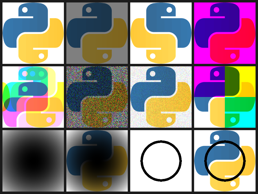

Core concepts

Concept 1 — Channel ops and slice operators

Three of the cheapest, most expressive transformations are pure slicing:

• Brightness — a // 2 halves every value. Multiplication scales each pixel’s intensity uniformly.
• Flip — a[:, ::-1] reverses the column axis. ::-1 is NumPy’s “every row/column, but in reverse” slice. Free; no allocation, just a view.
• Channel kill — g[:, :, 1] = 0 zeroes the green channel in-place. RGB minus green is roughly the magenta-purple range you see in the second tile of the grid above.

These three operators share a property: the operator commutes with broadcasting. You can apply a // 2 to a single image, a batch of images, an animation frame, or a video tensor — the code is identical. That broadcast-friendliness is what makes NumPy operations the natural building blocks of animation.

Concept 2 — Displacement with np.roll

np.roll(arr, k, axis=ax) shifts an array by k positions along an axis, wrapping the displaced elements around to the other end. Rolling a single channel produces a chromatic aberration-style effect:

roll = a.copy()
roll[:, :, 2] = np.roll(roll[:, :, 2], 25, axis=1)   # blue → +25 px right
roll[:, :, 1] = np.roll(roll[:, :, 1], 50, axis=0)   # green → +50 px down

Red stays in place; green and blue shift by different amounts. The same effect, with 25 replaced by int(25 * sin(time)), becomes the canonical “VHS glitch” animation in 8.2.4. The mechanical change between this lesson and that one is one line — 25 becomes int(25 * sin(t)).

Concept 3 — Distance fields and boolean masks

Many of the more dramatic transformations use a distance field: a 2D array where each entry is the (squared) distance from the corresponding pixel to a fixed centre point. Compute it once with np.mgrid:

yy, xx = np.mgrid[:H, :W]
cy, cx = H // 2, W // 2
circle = (xx - cx) ** 2 + (yy - cy) ** 2     # squared distance to centre

np.mgrid[:H, :W] is a one-line way to get two (H, W) arrays of row and column indices. The squared-distance arithmetic is then elementwise — every pixel knows its distance from the centre at the cost of one multiplication and one addition each.

The donut mask uses two thresholds on circle to isolate a thin ring:

donut = np.logical_and(circle < 4500, circle > 3500)
mask = 1 - donut.astype(np.int64)         # 0 inside the ring, 1 outside
# Multiply each channel by mask → ring punched out of the image

Same boolean-mask paradigm you saw with the Mandelbrot iteration (4.1.3); same np.mgrid you saw with the vector fields in 2.2.3. The distance field is the bridge between coordinate-grid maths and pixel-level rendering.

Exercises

Three exercises in Execute → Modify → Create order: run the full transformation pipeline, swap individual operators, then build a vignette from a distance field.

import numpy as np
from PIL import Image

def vignette(image, strength=1.0):
    """Return a new image with brightness fading from full at the centre
    to (1 - strength) at the corners."""
    H, W, _ = image.shape

    # TODO 1: build the squared-distance field with np.mgrid

    # TODO 2: normalise so the centre is 0 and the corners are 1

    # TODO 3: brightness factor = 1 - strength * normalised_distance
    #         (clip to [0, 1] to be safe)

    # TODO 4: multiply each channel by the brightness factor, return a uint8 image
    return image

a = np.array(Image.open('python_logo.png').convert('RGB'))
Image.fromarray(vignette(a, strength=0.85)).save('vignette.png')

yy, xx = np.mgrid[:H, :W]
cy, cx = H // 2, W // 2
dist = np.sqrt((xx - cx) ** 2 + (yy - cy) ** 2)
max_dist = np.sqrt(cx ** 2 + cy ** 2)
norm = dist / max_dist                       # 0 at centre, 1 at corners

brightness = np.clip(1.0 - strength * norm, 0, 1)
out = image.astype(np.float32) * brightness[..., None]   # broadcast over channels
return out.clip(0, 255).astype(np.uint8)

import numpy as np
from PIL import Image

def vignette(image, strength=1.0):
    H, W, _ = image.shape
    yy, xx = np.mgrid[:H, :W]
    cy, cx = H // 2, W // 2
    dist = np.sqrt((xx - cx) ** 2 + (yy - cy) ** 2)
    max_dist = np.sqrt(cx ** 2 + cy ** 2)
    norm = dist / max_dist
    brightness = np.clip(1.0 - strength * norm, 0, 1)
    out = image.astype(np.float32) * brightness[..., None]
    return out.clip(0, 255).astype(np.uint8)

a = np.array(Image.open('python_logo.png').convert('RGB'))
Image.fromarray(vignette(a, strength=0.85)).save('vignette.png')

Downloads

Summary

Common pitfalls to avoid

• Forgetting .copy() before mutating. g = a; g[:, :, 1] = 0 modifies a in place because g is just a view. Use a.copy().
• Overflow in uint8 arithmetic. a * a on uint8 wraps around at 256. Cast to int64 or float32 before multiplying, then clip and cast back.
• np.roll without an axis argument. Defaults to flattening the array first; the shift is then per-element across the entire raster, not per-axis. Always specify axis=0 or axis=1.
• Square-root distances when you only need to compare. Use squared distances for thresholding; reserve sqrt for displays where the visual falloff matters.

References

- [1] Muybridge, E. (1887). Animal Locomotion: An Electro-Photographic Investigation of Consecutive Phases of Animal Movements. University of Pennsylvania.
- [2] Born, M., & Wolf, E. (1999). Principles of Optics: Electromagnetic Theory of Propagation, Interference and Diffraction of Light (7th ed.). Cambridge University Press. ISBN 978-0-521-64222-4.
- [3] Gonzalez, R. C., & Woods, R. E. (2018). Digital Image Processing (4th ed.). Pearson. ISBN 978-0-13-335672-4.
- [4] Harris, C. R., Millman, K. J., van der Walt, S. J., et al. (2020). Array programming with NumPy. Nature, 585, 357–362. doi:10.1038/s41586-020-2649-2
- [5] Foley, J. D., van Dam, A., Feiner, S. K., & Hughes, J. F. (1990). Computer Graphics: Principles and Practice (2nd ed.). Addison-Wesley. ISBN 978-0-201-12110-0.
- [6] NumPy Community. (2024). numpy.roll. NumPy Documentation. numpy.org/roll
- [7] Pearson, M. (2011). Generative Art: A Practical Guide Using Processing. Manning. ISBN 978-1-935182-62-5.