2.1.3 Drawing Circles

Overview

A circle is defined by one number: how far you stand from a fixed point. Move along the boundary and the radius does not change. Translated into pixel arithmetic, that single fact becomes a one-line image — compare each pixel’s squared distance from a centre to the squared radius, and the boundary falls out as a boolean mask [1]. In this lesson you will build that mask with np.ogrid, swap the colour with one assignment, then iterate the same pattern into bull’s-eyes and gradient rings.

Learning objectives

1. Define a circle in terms of the Euclidean distance formula, $(x - c_x)^2 + (y - c_y)^2 < r^2$.
2. Use np.ogrid to build memory-efficient coordinate grids and leverage broadcasting for whole-image arithmetic.
3. Apply boolean masking to colour exactly the pixels that satisfy a geometric condition.
4. Layer concentric circles — drawn largest-first — to produce the classic bull’s-eye pattern.

Quick start — one orange disc

import numpy as np
from PIL import Image

CANVAS_SIZE = 512
CENTER_X, CENTER_Y = 256, 256
RADIUS = 150
CIRCLE_COLOR = [255, 128, 0]   # orange

# Open coordinate grids — Y is (512, 1), X is (1, 512)
Y, X = np.ogrid[0:CANVAS_SIZE, 0:CANVAS_SIZE]

# Squared distance from centre for every pixel
square_distance = (X - CENTER_X) ** 2 + (Y - CENTER_Y) ** 2

# Boolean mask of pixels inside the circle
inside_circle = square_distance < RADIUS ** 2

canvas = np.zeros((CANVAS_SIZE, CANVAS_SIZE, 3), dtype=np.uint8)
canvas[inside_circle] = CIRCLE_COLOR

Image.fromarray(canvas, mode='RGB').save('circle.png')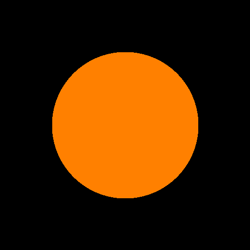

Core concepts

Concept 1 — Distance is enough

A circle is the locus of points at a fixed distance from a centre. For a centre $(c_x, c_y)$ and radius $r$, a pixel at $(x, y)$ is inside when

sqrt((x - cx)² + (y - cy)²) < r.

The square root is honest but expensive. Square both sides and the comparison becomes

(x - cx)² + (y - cy)² < r²,

which uses only multiplications and one subtraction per pixel. For the test d < r (with both sides non-negative) and d² < r² are equivalent — but the squared form is what every fast circle rasterizer reaches for, from Bresenham’s 1977 integer arc algorithm onward [2].

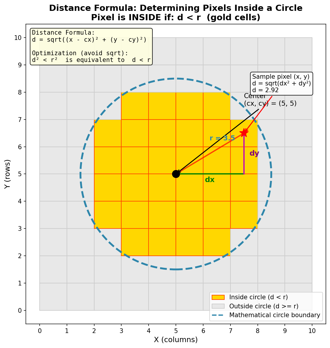
Concept 2 — np.ogrid is the cheap coordinate grid

To run arithmetic per pixel, you need arrays that hold each pixel’s coordinates. np.ogrid produces these as open grids — one column vector, one row vector — and lets broadcasting expand them to the full plane on demand:

import numpy as np

Y, X = np.ogrid[0:512, 0:512]
# Y.shape → (512, 1), values 0..511 as a column vector
# X.shape → (1, 512), values 0..511 as a row vector

# Broadcasting expands both to (512, 512) on demand
square_distance = (X - 256) ** 2 + (Y - 256) ** 2
# square_distance.shape → (512, 512)

The alternatives are real options but heavier. np.meshgrid materialises both arrays as full 2D grids (twice the memory). np.indices builds a 3D stack of coordinates. For circles, ogrid is the lightest tool that does the job [3].

Concept 3 — Boolean masks as paint stencils

square_distance < RADIUS ** 2 returns a 2D boolean array of the same shape as the canvas. That array is a mask — wherever it is True, the next assignment writes; wherever it is False, the original pixel survives:

canvas = np.zeros((512, 512, 3), dtype=np.uint8)
canvas[inside_circle] = [255, 128, 0]   # only True positions get coloured

This is boolean indexing (sometimes called fancy indexing). The mask broadcasts across the colour-channel axis automatically, so a 2D mask can paint into a 3D (H, W, 3) canvas without any extra reshape [4].

Exercises

Three exercises in Execute → Modify → Create order: run the basic circle, vary its parameters, then build a bull’s-eye from scratch.

import numpy as np
from PIL import Image

CANVAS_SIZE = 512
CENTER_X, CENTER_Y = 256, 256
RADIUS = 150
CIRCLE_COLOR = [255, 128, 0]

Y, X = np.ogrid[0:CANVAS_SIZE, 0:CANVAS_SIZE]
square_distance = (X - CENTER_X) ** 2 + (Y - CENTER_Y) ** 2
inside_circle = square_distance < RADIUS ** 2

canvas = np.zeros((CANVAS_SIZE, CANVAS_SIZE, 3), dtype=np.uint8)
canvas[inside_circle] = CIRCLE_COLOR

Image.fromarray(canvas, mode='RGB').save('circle.png')

MODIFY II.

Three colour and placement variations

Edit exercise1_execute.py to produce these images.

Goals

1. Small top-left circle — radius 50 centred near (100, 100).
2. Blue circle — same shape, but pure blue rather than orange.
3. Two circles side by side — red on the left, green on the right, both radius 100.

Goal 1 — what to expect

Change two lines:

CENTER_X, CENTER_Y = 100, 100
RADIUS = 50

The disc shrinks and shifts to the upper-left corner; everything else stays the same.

Goal 2 — what to expect

Swap the colour for [0, 0, 255]. RGB is [red, green, blue], so the third channel is what controls blueness:

CIRCLE_COLOR = [0, 0, 255]

Goal 3 — what to expect

Two square_distance computations and two mask assignments — one per circle. They are independent: the only shared state is the canvas they paint into.

dist1 = (X - 150) ** 2 + (Y - 256) ** 2
canvas[dist1 < 100 ** 2] = [255, 0, 0]

dist2 = (X - 360) ** 2 + (Y - 256) ** 2
canvas[dist2 < 100 ** 2] = [0, 255, 0]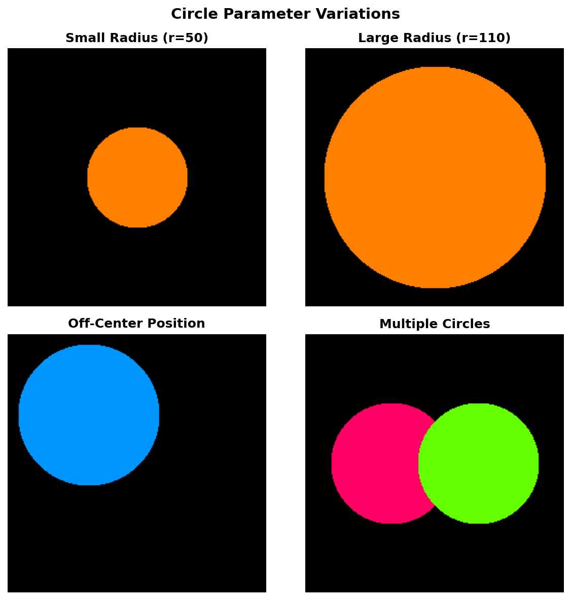

CREATE III.

Bull's-eye with concentric rings

Build a bull’s-eye: five concentric circles, alternating red and white, drawn around a single centre.

Goal: on a 512×512 canvas centred at (256, 256), draw circles of radii 200, 160, 120, 80, 40 in the colour sequence red, white, red, white, red (outermost to innermost).

python · exercise3_starter.py Copy

import numpy as np
from PIL import Image

CANVAS_SIZE = 512
CENTER_X, CENTER_Y = 256, 256

RADII  = [200, 160, 120, 80, 40]
RED, WHITE = [255, 0, 0], [255, 255, 255]
COLORS = [RED, WHITE, RED, WHITE, RED]

Y, X = np.ogrid[0:CANVAS_SIZE, 0:CANVAS_SIZE]
square_distance = (X - CENTER_X) ** 2 + (Y - CENTER_Y) ** 2

canvas = np.zeros((CANVAS_SIZE, CANVAS_SIZE, 3), dtype=np.uint8)

# TODO 1: loop over (radius, color) pairs from RADII and COLORS.
# TODO 2: for each pair, build the boolean mask square_distance < radius ** 2
#         and assign the colour into canvas at the mask.

# Hint: the order of the loop matters. Draw the largest circle first.

Image.fromarray(canvas, mode='RGB').save('concentric_circles.png')

Hint 1 — why largest first

Each iteration overwrites everything inside the current mask. If you draw the smallest circle first and then a larger one on top, the larger circle paints over the smaller one and you only see one ring. Painting largest-to-smallest produces the bull’s-eye automatically — same painter’s algorithm idea as in the triangle landscape.

Hint 2 — iterating two lists in lockstep

zip pairs items from each list one for one:

for radius, color in zip(RADII, COLORS):
    mask = square_distance < radius ** 2
    canvas[mask] = color

The lists are already in largest-to-smallest order, so the loop just walks them.

Complete solution

python · exercise3_solution.py Copy

import numpy as np
from PIL import Image

CANVAS_SIZE = 512
CENTER_X, CENTER_Y = 256, 256

RADII  = [200, 160, 120, 80, 40]
RED, WHITE = [255, 0, 0], [255, 255, 255]
COLORS = [RED, WHITE, RED, WHITE, RED]

Y, X = np.ogrid[0:CANVAS_SIZE, 0:CANVAS_SIZE]
square_distance = (X - CENTER_X) ** 2 + (Y - CENTER_Y) ** 2

canvas = np.zeros((CANVAS_SIZE, CANVAS_SIZE, 3), dtype=np.uint8)
for radius, color in zip(RADII, COLORS):
    canvas[square_distance < radius ** 2] = color

Image.fromarray(canvas, mode='RGB').save('concentric_circles.png')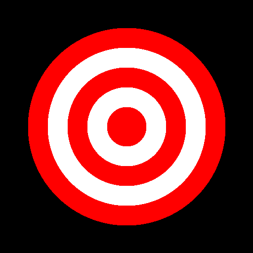

How it works:

• square_distance is computed once, outside the loop. Every iteration reuses the same scalar field.
• zip(RADII, COLORS) walks the two lists in parallel — radius 200 with red, then 160 with white, and so on.
• Drawing in that order means each subsequent (smaller) circle overwrites the inside of the previous (larger) one, leaving an alternating ring pattern.

Make it your own

• Gradient rings. Replace the discrete COLORS list with np.linspace-interpolated colours across 20+ thin rings.
• Off-centre tunnel. Shift each successive circle’s centre by (dx, dy) = (i*4, i*2) to fake a perspective tunnel.
• Four-petal flower. Place four circles around a central point at the cardinal directions, all the same radius, and watch their intersections form a quatrefoil.

Downloads

Summary

Common pitfalls to avoid

• Comparing square_distance < RADIUS instead of RADIUS ** 2 — produces a tiny dot because you forgot to square the right side.
• Drawing concentric circles smallest-first — the larger circle paints over the smaller ones and the bull’s-eye collapses to one solid disc.
• Using np.meshgrid reflexively — works fine, but uses more memory than np.ogrid when you only need broadcasting.
• Integer overflow on very large canvases — (X - cx)**2 in int32 can wrap around for cx, X near the edges of a multi-thousand-pixel canvas; cast to int64 or float64 for safety.

References

- [1] Foley, J. D., van Dam, A., Feiner, S. K., & Hughes, J. F. (1990). Computer Graphics: Principles and Practice (2nd ed.). Addison-Wesley.
- [2] Bresenham, J. E. (1977). A linear algorithm for incremental digital display of circular arcs. Communications of the ACM, 20(2), 100–106. doi:10.1145/359423.359432
- [3] NumPy Community. (2024). numpy.ogrid. NumPy Documentation. numpy.org
- [4] Harris, C. R., et al. (2020). Array programming with NumPy. Nature, 585(7825), 357–362. doi:10.1038/s41586-020-2649-2
- [5] Gonzalez, R. C., & Woods, R. E. (2018). Digital Image Processing (4th ed.). Pearson.
- [6] Pearson, M. (2011). Generative Art: A Practical Guide Using Processing. Manning.
- [7] Paas, F., & van Merriënboer, J. J. G. (2020). Cognitive-load theory: Methods to manage working memory load in the learning of complex tasks. Current Directions in Psychological Science, 29(4), 394–398. doi:10.1177/0963721420922183