2.2.3 Vector Fields

Overview

A vector field assigns a direction to every point in space — wind across a weather map, water in a current, the gravity vector pointing back toward Earth’s centre [1]. Most of those fields are invisible. Visualising one is the inverse problem: take (dx, dy) per pixel, recover the angle with np.arctan2, then map angle to hue on the colour wheel. The result is a pattern where colour reveals direction, and combining a few simple fields — radial in, radial out, rotational — gives you vortexes, spirals, and the whole vocabulary of fluid-style flow.

Learning objectives

1. Define a vector field as a function that assigns (dx, dy) to every coordinate.
2. Recover direction from a vector using np.arctan2(dy, dx), which handles all four quadrants without division-by-zero.
3. Map an angle in [-π, π] to a hue in [0, 255] and render it as a colour wheel.
4. Compose new fields by adding radial and rotational components — the building blocks of vortexes and spirals.

Quick start — a radial vector field

import numpy as np
from PIL import Image

def hue_to_rgb(hue):
    """Map an array of hue values in [0, 1] to RGB via the standard 6-segment wheel."""
    h6 = hue * 6
    c = np.ones_like(h6)
    x = 1 - np.abs((h6 % 2) - 1)
    z = np.zeros_like(h6)
    seg = h6.astype(int)
    r = np.choose(seg % 6, [c, x, z, z, x, c])
    g = np.choose(seg % 6, [x, c, c, x, z, z])
    b = np.choose(seg % 6, [z, z, x, c, c, x])
    return (np.stack([r, g, b], axis=-1) * 255).astype(np.uint8)

H, W = 512, 512
cx, cy = W // 2, H // 2

y, x = np.ogrid[:H, :W]
dx = cx - x           # vector pointing toward centre
dy = cy - y

angle = np.arctan2(dy, dx)                  # in [-pi, pi]
hue = (angle + np.pi) / (2 * np.pi)         # in [0, 1]
rgb = hue_to_rgb(np.broadcast_to(hue, (H, W)))

Image.fromarray(rgb, mode='RGB').save('simple_vector_field.png')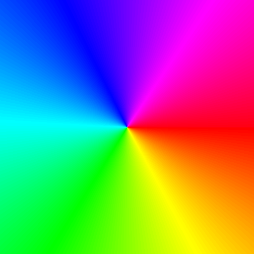

Core concepts

Concept 1 — Vector fields and arctan2

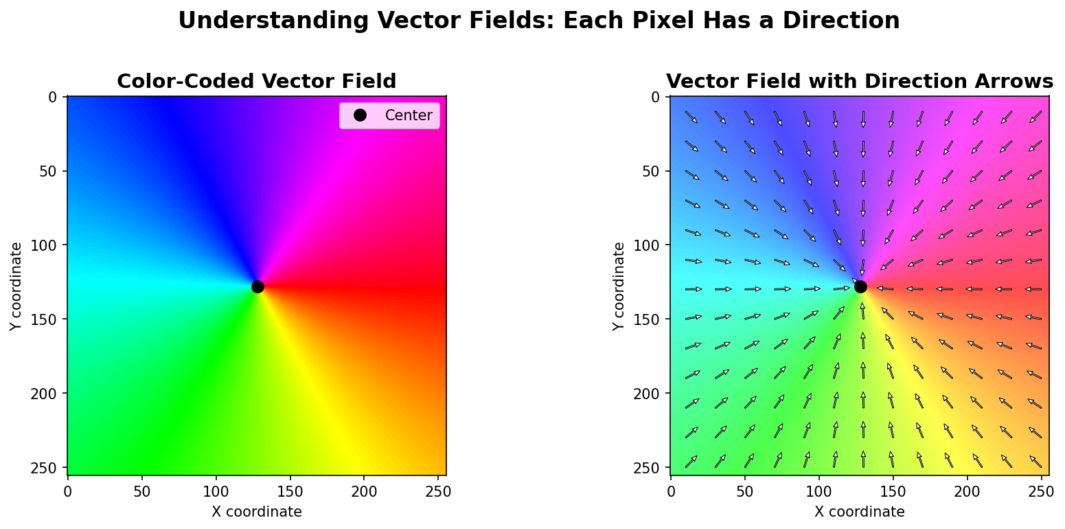
A vector field is a function F(x, y) = (dx, dy) that assigns a 2D vector to every point. The radial-in field is F(x, y) = (cx - x, cy - y): at every pixel, an arrow pointing toward the centre. The rotational field is its 90° rotation: swap and negate. Combine them and you get vortexes.

To turn a vector into a colour, you need its angle. The function for that is np.arctan2(dy, dx), which returns the angle in [-π, π] and handles every quadrant correctly:

import numpy as np

# (1, 1) → π/4 (up-right)
print(np.arctan2(1, 1))     # 0.7854

# (-1, 1) → 3π/4 (up-left)
print(np.arctan2(1, -1))    # 2.3562

# (0, 0) → 0 (undefined direction; convention picks 0)
print(np.arctan2(0, 0))     # 0.0

Crucially, arctan2(dy, dx) is not the same as arctan(dy/dx). The latter loses sign information (a 180° flip in both dx and dy gives the same ratio), throws on dx = 0, and collapses two quadrants into one. Always use arctan2 for direction calculations [3].

Concept 2 — Mapping angle to hue

arctan2 returns values in [-π, π]. The colour-wheel convention treats hue as cyclic in [0, 1] (or [0, 360°]). The mapping is two arithmetic steps:

hue = (θ + π) / (2π).

This shifts and rescales: -π goes to 0 (red), 0 goes to 0.5 (cyan), +π goes back to 1 (red again — the wheel wraps). Once you have hue in [0, 1], a small hue_to_rgb helper walks the standard six-segment HSV wheel: red → yellow → green → cyan → blue → magenta → red [4].

Concept 3 — Composing radial and rotational fields

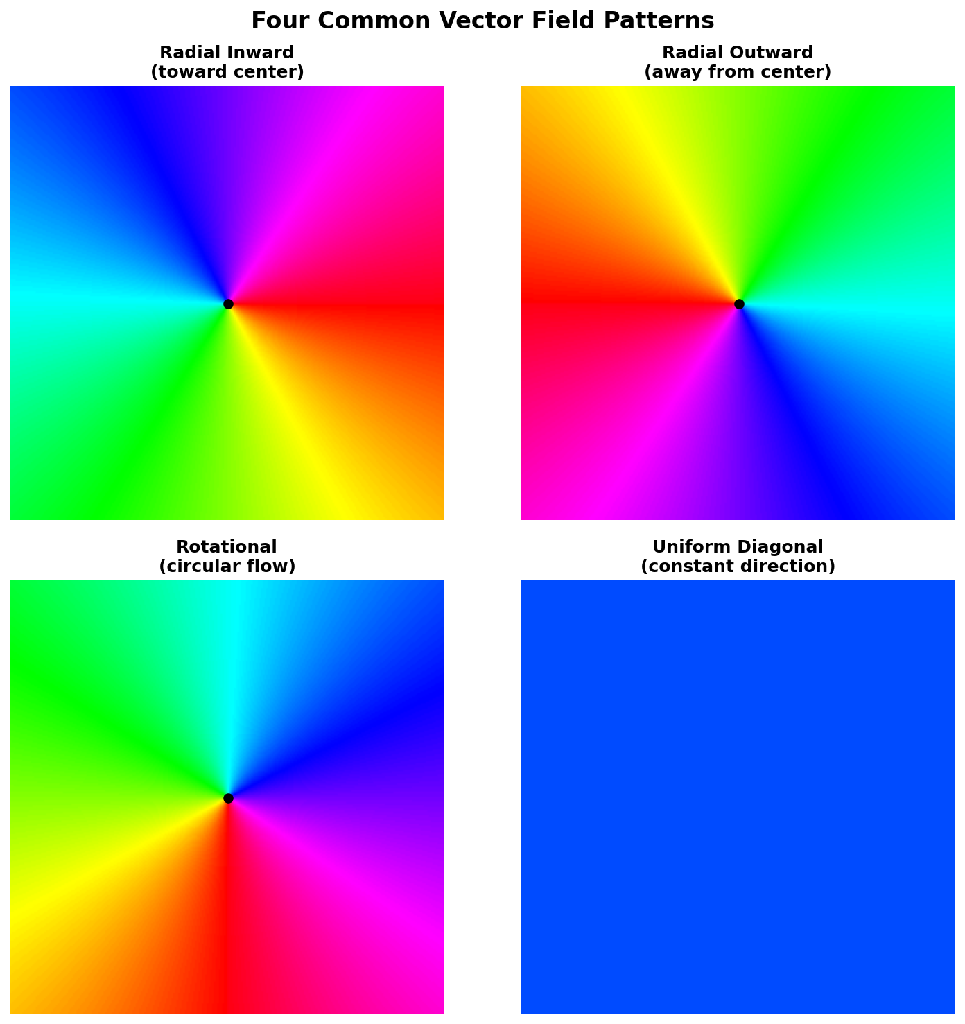
Three primitives compose almost every flow you will see:

• Radial inward — dx = cx - x, dy = cy - y. Vectors point at the centre. Looks like gravity.
• Radial outward — dx = x - cx, dy = y - cy. The reverse. Looks like an explosion.
• Rotational — perpendicular to radial. Counterclockwise: dx = -(y - cy), dy = (x - cx). Looks like a whirlpool’s surface.

Adding components produces vortexes:

rel_x = x - cx
rel_y = y - cy

dx_rot, dy_rot = -rel_y,  rel_x        # rotation (CCW)
dx_rad, dy_rad = -rel_x, -rel_y        # radial inward

dx = 0.7 * dx_rot + 0.3 * dx_rad
dy = 0.7 * dy_rot + 0.3 * dy_rad

The weights set the character: 100% rotation gives clean circular flow; 100% inward gives a sink; 70/30 gives the spiral pull of a draining bath or a hurricane seen from above. Maxwell’s equations describe real electromagnetic fields the same way — as superpositions of simple radial and rotational components [5].

Exercises

Three exercises in Execute → Modify → Create order: run the radial field, swap to outward and rotational, then build a weighted vortex.

MODIFY II.

Outward, rotational, spiral

Edit the quick-start code (only the dx, dy lines) to produce these three pictures.

Goals

1. Outward — vectors point away from the centre.
2. Rotational (counterclockwise) — vectors are perpendicular to the radial-out direction.
3. Spiral — outward + rotational combined (just add the components).

Goal 1 — what to expect

Reverse the subtraction:

dx = x - cx
dy = y - cy

Every colour appears 180° from where it did in the inward field — the rainbow rotates a half-turn around the centre.

Goal 2 — what to expect

Swap and negate one component:

rel_x = x - cx
rel_y = y - cy
dx = -rel_y
dy =  rel_x

The colours form concentric bands around the centre instead of radial wedges — the field is tangent to circles.

Goal 3 — what to expect

Add the two (dx, dy) pairs:

rel_x = x - cx
rel_y = y - cy
dx = -rel_y + rel_x         # rotation + outward
dy =  rel_x + rel_y

The colour bands twist — every step rotates as it moves outward, which is exactly the visual of a spiral.

CREATE III.

Vortex with weighted components

Build a vortex: 70% rotation, 30% inward radial. Normalise the radial component so the inward pull is consistent across the canvas, regardless of distance from the centre.

python · exercise3_starter.py Copy

import numpy as np
from PIL import Image

# ... hue_to_rgb helper from quick start ...

H, W = 512, 512
cx, cy = W // 2, H // 2

y, x = np.ogrid[:H, :W]
rel_x = x - cx
rel_y = y - cy

distance = np.sqrt(rel_x ** 2 + rel_y ** 2)
distance[distance == 0] = 1     # avoid 0/0 at the centre

# TODO 1: build the rotational component (perpendicular to radial)
# dx_rot, dy_rot = ...

# TODO 2: build the *normalised* radial inward component
# dx_rad = -rel_x / distance
# dy_rad = -rel_y / distance

# TODO 3: combine with 70% rotation and 30% radial. Multiply the radial
# part by `distance` in the sum so the rotation dominates near the centre.

# TODO 4: compute angle = arctan2(dy_combined, dx_combined),
# then hue and RGB as in the quick start.

Image.fromarray(rgb, mode='RGB').save('vortex_field.png')

Hint — combining the components

dx_rot, dy_rot = -rel_y, rel_x
dx_rad = -rel_x / distance
dy_rad = -rel_y / distance

w_rot, w_rad = 0.7, 0.3
dx = w_rot * dx_rot + w_rad * dx_rad * distance
dy = w_rot * dy_rot + w_rad * dy_rad * distance

The * distance on the radial term un-does the normalisation — it lets the rotation dominate near the centre (where everything is small) without exploding the radial term to enormous values far away.

Complete solution

python · exercise3_solution.py Copy

import numpy as np
from PIL import Image

def hue_to_rgb(hue):
    h6 = hue * 6
    c = np.ones_like(h6); z = np.zeros_like(h6)
    x = 1 - np.abs((h6 % 2) - 1)
    seg = h6.astype(int)
    r = np.choose(seg % 6, [c, x, z, z, x, c])
    g = np.choose(seg % 6, [x, c, c, x, z, z])
    b = np.choose(seg % 6, [z, z, x, c, c, x])
    return (np.stack([r, g, b], axis=-1) * 255).astype(np.uint8)

H, W = 512, 512
cx, cy = W // 2, H // 2

y, x = np.ogrid[:H, :W]
rel_x = x - cx
rel_y = y - cy
distance = np.sqrt(rel_x ** 2 + rel_y ** 2)
distance[distance == 0] = 1

dx_rot, dy_rot = -rel_y, rel_x
dx_rad = -rel_x / distance
dy_rad = -rel_y / distance

w_rot, w_rad = 0.7, 0.3
dx = w_rot * dx_rot + w_rad * dx_rad * distance
dy = w_rot * dy_rot + w_rad * dy_rad * distance

angle = np.arctan2(dy, dx)
hue = (angle + np.pi) / (2 * np.pi)
rgb = hue_to_rgb(np.broadcast_to(hue, (H, W)))

Image.fromarray(rgb, mode='RGB').save('vortex_field.png')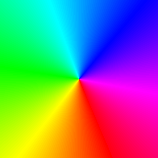

How it works:

• The rotational component (-rel_y, rel_x) is the counterclockwise tangent.
• The radial component is normalised (/ distance), which would make the centre singular without the distance[distance == 0] = 1 guard.
• Multiplying the radial part by distance in the sum un-does the normalisation in a controlled way — this prevents the radial pull from blowing up the rotation near the edges.
• arctan2 of the combined field gives the angle at every pixel; hue_to_rgb paints it.

Make it your own

• 90/10 vortex. Almost pure rotation, with a barely-noticeable inward pull. The bands curl very gently — looks like a slow eddy.
• Saddle. Mix radial outward in one axis and radial inward in the other: dx = x - cx, dy = cy - y. The colour field shows the classic four-quadrant saddle pattern from dynamical systems.
• Sin/cos field. Replace (dx, dy) with (sin(y/40), cos(x/40)). A non-radial pattern that looks like a fluid-dynamics simulation snapshot.

Downloads

Summary

Common pitfalls to avoid

• np.arctan(dy / dx) instead of np.arctan2(dy, dx) — drops the sign of (dx, dy), throws on dx = 0, collapses two quadrants.
• Forgetting that arctan2 returns [-π, π] and not normalising before computing hue — the rainbow ends up shifted by half a turn.
• Dividing by distance without guarding distance == 0 — silent NaNs propagate through the entire image.
• Mismatched broadcasting: if your dx, dy aren’t both (H, W) after broadcasting, arctan2 will broadcast in an unexpected direction.

References

- [1] Acheson, D. J. (1990). Elementary Fluid Dynamics. Oxford University Press.
- [2] Laidlaw, D. H., & Weickert, J. (Eds.). (2005). Visualization and Processing of Tensor Fields. Springer.
- [3] NumPy Community. (2024). numpy.arctan2. NumPy Documentation. numpy.org
- [4] Smith, A. R. (1978). Color gamut transform pairs. ACM SIGGRAPH Computer Graphics, 12(3), 12–19. doi:10.1145/965139.807361
- [5] Maxwell, J. C. (1865). A dynamical theory of the electromagnetic field. Philosophical Transactions of the Royal Society of London, 155, 459–512.
- [6] Bridson, R. (2015). Fluid Simulation for Computer Graphics (2nd ed.). CRC Press.
- [7] Harris, C. R., et al. (2020). Array programming with NumPy. Nature, 585(7825), 357–362. doi:10.1038/s41586-020-2649-2