2.3.3 Harmonograph Simulation
Add exponential damping to two perpendicular sinusoids and the Lissajous figures from the previous lesson start to spiral inward — the same effect that gives Victorian harmonographs their characteristic decaying motion.
Overview
A harmonograph is a Victorian drawing machine — two pendulums, one driving the pen along x and the other along y, leaving an ink trace on a sheet of paper [1]. The two pendulums oscillate at slightly different frequencies and lose energy slowly to friction, so the resulting trace is a Lissajous figure that spirals inward as the swings die out. Mathematically you add one factor to the Lissajous equations from 2.3.1 — an exponential decay exp(-d·t) — and the curve picks up that same drift toward the centre. The harmonograph belongs to a pattern you will meet again throughout this module: complex behaviour emerging from two simple oscillations plus a slow dissipation.
Learning objectives
- Extend the Lissajous parametric equations with exponential damping
exp(-d·t)to model real pendulum decay. - Predict the basic harmonograph pattern from the frequency ratio (the musical interval analogy).
- Tune the damping coefficient
dto control how fast the pattern spirals into the centre. - Interpolate stroke colour by the decay factor to visualise energy dissipation along the curve.
Quick start — a 3:2 harmonograph
import numpy as np
from PIL import Image, ImageDraw

CANVAS_SIZE = 512
CENTER = CANVAS_SIZE // 2

# Two pendulums — X and Y
FREQ_X, AMP_X, PHASE_X = 3, 200, 0
FREQ_Y, AMP_Y, PHASE_Y = 2, 200, np.pi / 2

DAMPING = 0.002

t = np.linspace(0, 100, 5000)
decay = np.exp(-DAMPING * t)

x = CENTER + AMP_X * np.sin(FREQ_X * t + PHASE_X) * decay
y = CENTER + AMP_Y * np.sin(FREQ_Y * t + PHASE_Y) * decay

image = Image.new('RGB', (CANVAS_SIZE, CANVAS_SIZE), (10, 10, 20))
draw = ImageDraw.Draw(image)
points = list(zip(x.astype(int), y.astype(int)))
draw.line(points, fill=(100, 200, 255), width=1)
image.save('simple_harmonograph.png')
Core concepts
Concept 1 — Two damped pendulums
A pendulum swinging in real air loses a small fraction of its energy each cycle to friction. The textbook model is the damped sinusoid:
x(t) = A · sin(f·t + φ) · exp(-d·t), y(t) = B · sin(g·t + ψ) · exp(-d·t).
A, B are the amplitudes; f, g are the angular frequencies; φ, ψ are the phases; d is the damping coefficient. Without the e^{-dt} factor this is exactly the Lissajous parametric equation from 2.3.1. The exponential multiplier scales both axes uniformly — so the shape of the Lissajous figure stays the same; only its overall size shrinks with time [2].
t = np.linspace(0, 100, 5000)
decay = np.exp(-0.002 * t)        # exponential energy loss

x = 200 * np.sin(3 * t)              * decay
y = 200 * np.sin(2 * t + np.pi/2)    * decay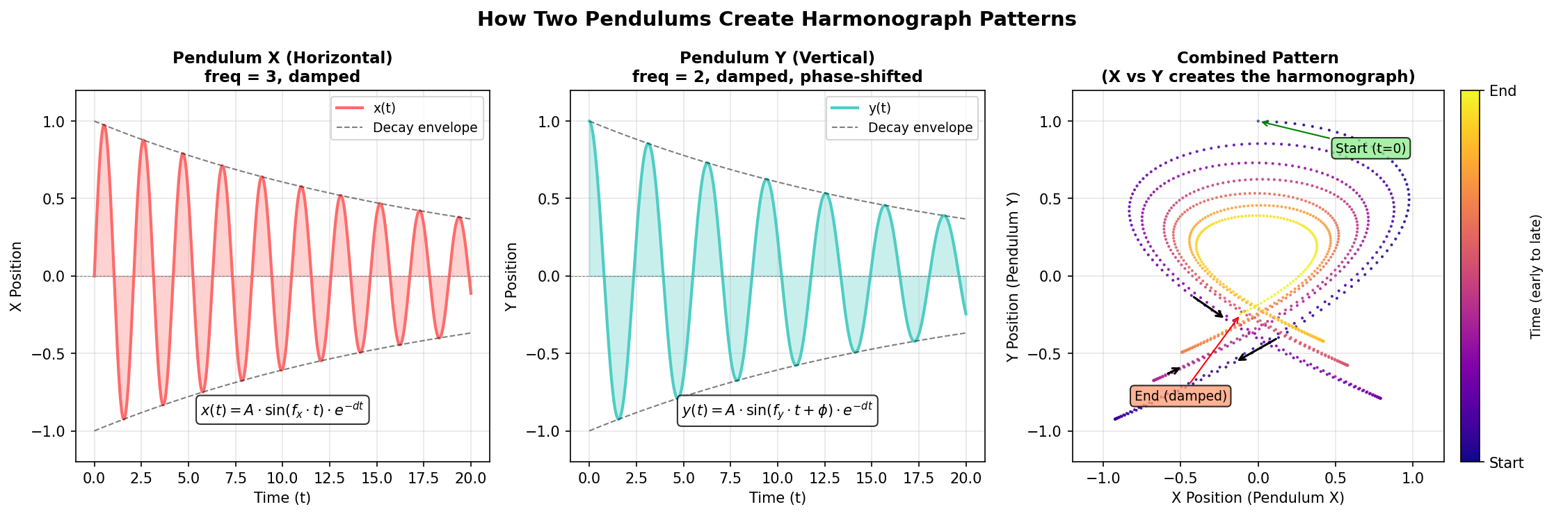
Concept 2 — Frequency ratios as musical intervals
The character of the pattern is determined almost entirely by the frequency ratio f : g. The match with music is no accident: a 3:2 frequency ratio sounds as a perfect fifth on a piano, and it traces as a three-lobed harmonograph. The Greeks called this correspondence the music of the spheres — small-integer frequency ratios are the same thing whether the medium is air pressure or pen position [1, 3].
| Ratio | Visual pattern | Musical interval |
|---|---|---|
| 1:1 | Circle or ellipse | Unison |
| 2:1 | Figure-8 | Octave |
| 3:2 | Three-lobe pattern | Perfect fifth |
| 4:3 | Four-lobe pattern | Perfect fourth |
| 5:4 | Five-lobe pattern | Major third |
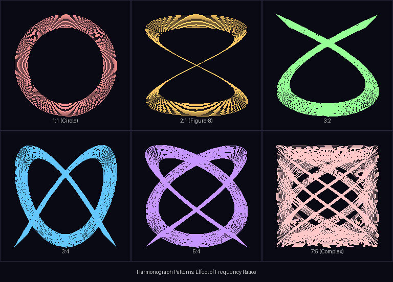
The simpler the ratio, the simpler the figure. Irrational ratios (say, f = √2) never close — the curve eventually fills its bounding rectangle just like an irrational Lissajous.
Concept 3 — Damping and the inward spiral
The damping coefficient d controls how fast both pendulums lose amplitude. With decay = exp(-d·t):
- t = 0 → decay = 1.0 (full amplitude).
- t = 1/d → decay ≈ 0.37 (one e-fold).
- t = 3/d → decay ≈ 0.05 (essentially at rest).
Three rough regimes for a t = 0..100 sweep:
- Low damping (d ≈ 0.001) — many loops trace before any visible shrinkage; the pattern fills its bounding rectangle.
- Medium damping (d ≈ 0.005) — clear spiral inward over the visible sweep; the pattern reads as a Lissajous slowly winding into the centre.
- High damping (d ≈ 0.01) — the pen reaches the centre well before the time sweep ends; only the first few cycles are visible.
Without damping, the same equations produce a normal (un-spiraling) Lissajous curve, traced indefinitely on top of itself [2].
for d in [0.001, 0.005, 0.01]:
    decay = np.exp(-d * t)
    # plot — slow / medium / fast spiral inward
Exercises
Three exercises in Execute → Modify → Create order: run a 3:2 harmonograph, swap frequency ratios and damping, then colour-fade the stroke by decay.
Run the 3:2 harmonograph
Run simple_harmonograph.py from the quick start. Inspect the output.
Reflection questions
- What frequency ratio is in the script, and how is that ratio visible in the picture?
- Where does the pattern begin (at
t = 0) and where does it end? - What would happen if
PHASE_Ywere set to0rather thanπ/2?
Answers
3:2 ratio — X completes three cycles for every two by Y. The resulting Lissajous has interlocking loops that you can count: roughly three “lobes” along the y-axis and two along the x-axis.
Start and end — decay = 1 at t = 0, so the pattern starts at the outer edge with the full 200-pixel amplitude. By t = 100, decay ≈ exp(-0.2) ≈ 0.82, so the pen reaches the centre when both amplitudes have decayed to roughly 18% of the start. The trace ends near the centre after many shrinking loops.
Phase = 0 — both pendulums start at their zero crossings simultaneously, so x(0) = y(0) = 0. With the same frequency they would trace a diagonal line; with different frequencies they trace a degenerate Lissajous (closing onto itself). The π/2 phase shift is what opens the loops into the classic harmonograph look.
Three pattern variations
Edit simple_harmonograph.py to produce these three pictures.
Goals
- Figure-8 — pick a frequency ratio that traces a figure-8.
- Five-lobe — pick a frequency ratio that produces a pattern with five visible lobes.
- Faster decay — increase the damping so the pattern collapses to the centre much sooner.
Goal 1 — what to expect
FREQ_X, FREQ_Y = 2, 12:1 is the octave ratio. X swings twice for every Y swing, tracing the classic figure-8.
Goal 2 — what to expect
FREQ_X, FREQ_Y = 5, 45:4 (a major third) gives a five-lobed pattern with intricate interior structure. Try 5:3 for a different five-lobe variant.
Goal 3 — what to expect
DAMPING = 0.01Roughly five times the previous damping. The pen reaches near-zero amplitude well before the time sweep ends — only the first few loops are visible.
Colour-fading harmonograph
Render the harmonograph with a stroke that fades from bright cyan to dark blue as the pendulum loses energy. Use the decay factor to drive the colour interpolation.
import numpy as np
from PIL import Image, ImageDraw

CANVAS_SIZE = 512
CENTER = CANVAS_SIZE // 2

START_COLOR = (100, 255, 255)   # bright cyan (full energy)
END_COLOR   = (20, 40, 80)      # dark blue (decayed)

def faded_color(decay_value):
    # TODO 1: interpolate between START_COLOR (decay = 1) and END_COLOR (decay → 0).
    # Result: tuple of three uint8s.
    pass

t = np.linspace(0, 100, 5000)
decay = np.exp(-0.003 * t)
x = CENTER + 200 * np.sin(5 * t) * decay
y = CENTER + 200 * np.sin(4 * t + np.pi / 2) * decay

image = Image.new('RGB', (CANVAS_SIZE, CANVAS_SIZE), (10, 10, 20))
draw = ImageDraw.Draw(image)

# TODO 2: per-segment loop: for each i, colour = faded_color(decay[i]),
# then draw.line from (x[i-1], y[i-1]) to (x[i], y[i]) with that colour.

image.save('colored_harmonograph.png')
Hint 1 — colour interpolation
decay goes from 1.0 (start) toward 0 (end). Use it directly as the interpolation parameter:
def faded_color(decay_value):
    r = int(START_COLOR[0] * decay_value + END_COLOR[0] * (1 - decay_value))
    g = int(START_COLOR[1] * decay_value + END_COLOR[1] * (1 - decay_value))
    b = int(START_COLOR[2] * decay_value + END_COLOR[2] * (1 - decay_value))
    return (r, g, b)
When decay_value = 1, you get pure START_COLOR; when decay_value = 0, pure END_COLOR; in between, a smooth mix.
Hint 2 — per-segment draw loop
for i in range(1, len(t)):
    color = faded_color(decay[i])
    draw.line([(int(x[i-1]), int(y[i-1])), (int(x[i]), int(y[i]))],
              fill=color, width=1)
One Pillow call per segment — slower than draw.line(points, fill=...) but the only way to put a different colour on each segment.
Complete solution
import numpy as np
from PIL import Image, ImageDraw

CANVAS_SIZE = 512
CENTER = CANVAS_SIZE // 2

START_COLOR = (100, 255, 255)
END_COLOR   = (20, 40, 80)

def faded_color(decay_value):
    r = int(START_COLOR[0] * decay_value + END_COLOR[0] * (1 - decay_value))
    g = int(START_COLOR[1] * decay_value + END_COLOR[1] * (1 - decay_value))
    b = int(START_COLOR[2] * decay_value + END_COLOR[2] * (1 - decay_value))
    return (r, g, b)

t = np.linspace(0, 100, 5000)
decay = np.exp(-0.003 * t)
x = CENTER + 200 * np.sin(5 * t) * decay
y = CENTER + 200 * np.sin(4 * t + np.pi / 2) * decay

image = Image.new('RGB', (CANVAS_SIZE, CANVAS_SIZE), (10, 10, 20))
draw = ImageDraw.Draw(image)

for i in range(1, len(t)):
    color = faded_color(decay[i])
    draw.line([(int(x[i-1]), int(y[i-1])), (int(x[i]), int(y[i]))],
              fill=color, width=1)

image.save('colored_harmonograph.png')
How it works:
decayis a per-sample array;decay[i]is the energy at pointialong the curve.faded_colordoes linear interpolation between two RGB triples — same routine as the colour gradient in 2.1.2’s mountain sky.- The per-segment loop applies a different colour to every short line segment. The cost is one Pillow call per segment, but the visual reward is the energy gradient.
Make it your own
- Three pendulums. Add a third frequency:
x = ... + AMP_Z * np.sin(FREQ_Z * t + PHASE_Z) * decay. The visual gains an extra layer of structure. - Musical scale. Render six harmonographs side by side with the frequency ratios of the major scale (1:1, 9:8, 5:4, 4:3, 3:2, 5:3, 15:8, 2:1).
- Animation. Render only the first
Npoints, thenN+50, thenN+100, … and assemble a GIF. The viewer watches the pendulums lose energy in real time.
Downloads
simple_harmonograph.py — 3:2 quick start harmonograph_variations.py — frequency-ratio panel colored_harmonograph_solution.py — colour-faded referenceSummary
Common pitfalls to avoid
- Both phases equal — the figure collapses to a diagonal line.
- Damping too high — the pattern collapses to a single point before any structure is traced.
- Damping zero — the curve traces the same Lissajous indefinitely on top of itself, no inward spiral.
- Too few sample points — high frequency ratios alias. 5000 points covers ratios up to about 7:5 cleanly.
References
- [1] Ashton, A. (2003). Harmonograph: A Visual Guide to the Mathematics of Music (2nd ed.). Walker & Company.
- [2] Cundy, H. M., & Rollett, A. P. (1961). Mathematical Models (2nd ed.). Oxford University Press.
- [3] Klemens, B. (2010). The harmonograph. Make Magazine, 23, 124–127.
- [4] Weisstein, E. W. (2024). Lissajous curve. MathWorld — A Wolfram Web Resource. mathworld.wolfram.com/LissajousCurve
- [5] NumPy Community. (2024). numpy.exp. NumPy Documentation. numpy.org
- [6] Pearson, M. (2011). Generative Art: A Practical Guide Using Processing. Manning.
- [7] Foley, J. D., van Dam, A., Feiner, S. K., & Hughes, J. F. (1990). Computer Graphics: Principles and Practice (2nd ed.). Addison-Wesley.