2.2.4 Distance Fields & SDFs
Keep the actual distance values instead of thresholding them. Subtract a radius to get a signed distance function, then combine SDFs with `min`, `max`, and negation — the algebra behind modern shape composition.
Overview
In 2.1.3 you drew a circle by thresholding a distance — square_distance < r² gave a boolean mask and you threw the actual distance values away. Keep them instead and you have a distance field: a 2D scalar where each pixel stores the distance to the nearest point on a shape. Subtract the radius and you have a signed distance function (SDF): negative inside, positive outside, zero on the boundary [1]. The payoff is composition — three operations (min, max, and negation) let you take unions, intersections, and subtractions of any two SDFs, which is how modern font renderers, demoscene shaders, and Pixar’s recent shape pipelines do CSG without ever building polygons [2, 3].
Learning objectives
- Compute and visualise an unsigned distance field — the actual distance from every pixel to a centre point.
- Convert a distance field into a signed distance function by subtracting the shape’s defining parameter (e.g. a radius).
- Compose SDFs with
np.minimum(union),np.maximum(intersection), and negation (subtraction). - Build a multi-shape composition by combining circle and rectangle SDFs.
Quick start — a distance field from one centre
import numpy as np
from PIL import Image

SIZE = 512
CENTER_X, CENTER_Y = 256, 256

Y, X = np.ogrid[0:SIZE, 0:SIZE]

# Distance from every pixel to the centre (no threshold this time)
distance_field = np.sqrt((X - CENTER_X) ** 2 + (Y - CENTER_Y) ** 2)

# Normalise to [0, 255] for grayscale display
normalized = (distance_field / distance_field.max() * 255).astype(np.uint8)

Image.fromarray(normalized, mode='L').save('simple_distance_field.png')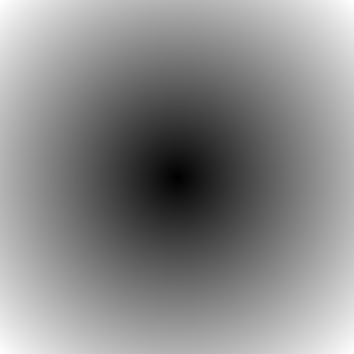
Core concepts
Concept 1 — Distance field vs. boolean mask
The circle code in 2.1.3 was
inside = (X - cx) ** 2 + (Y - cy) ** 2 < radius ** 2 # bool arrayThe distance-field version drops the comparison and keeps the floats:
distance = np.sqrt((X - cx) ** 2 + (Y - cy) ** 2) # float arrayA boolean tells you whether a pixel is in the shape. A distance tells you how far it is from the boundary. The continuous information enables:
- Soft edges — fade colour smoothly near the boundary rather than snapping.
- Collision queries — not just “is there overlap?” but “how much room is left?”
- Procedural texture — use the distance to drive a colour map, a sine wave (concentric rings), or a transparency curve [4].
Concept 2 — Signed distance functions
Subtracting the shape’s defining parameter turns a distance field into a signed one. For a circle of radius r:
SDF_circle(x, y) = sqrt((x - cx)² + (y - cy)²) - r
SDF < 0— inside the shape.SDF = 0— on the boundary.SDF > 0— outside.
distance = np.sqrt((X - cx) ** 2 + (Y - cy) ** 2)
circle_sdf = distance - radius        # negative inside, positive outside
The “signed” part is what makes composition work. With unsigned distance you can only test “near the shape”; with signed distance you can test “inside” and “outside” separately, and combine those tests algebraically [2].
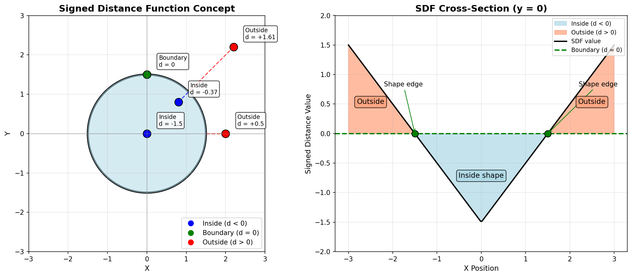
Concept 3 — Composing SDFs with min, max, and negation
The whole CSG (Constructive Solid Geometry) toolkit collapses to three NumPy operations on SDFs [2]:
| Operation | Formula | Intuition |
|---|---|---|
| Union (A ∪ B) | np.minimum(sdfA, sdfB) | The closer of the two — inside if inside either |
| Intersection (A ∩ B) | np.maximum(sdfA, sdfB) | The farther — inside if inside both |
| Subtraction (A − B) | np.maximum(sdfA, -sdfB) | Inside A and outside B |
min is correct for union because the SDF of the union should be negative wherever any component is negative — i.e. wherever the minimum of the components is negative. max is correct for intersection by the same reasoning with the sign flipped. Negating an SDF swaps inside and outside, which is what subtraction needs.
circle1 = np.sqrt(x ** 2 + y ** 2) - 80
circle2 = np.sqrt((x - 60) ** 2 + y ** 2) - 80

union        = np.minimum(circle1, circle2)
intersection = np.maximum(circle1, circle2)
subtraction  = np.maximum(circle1, -circle2)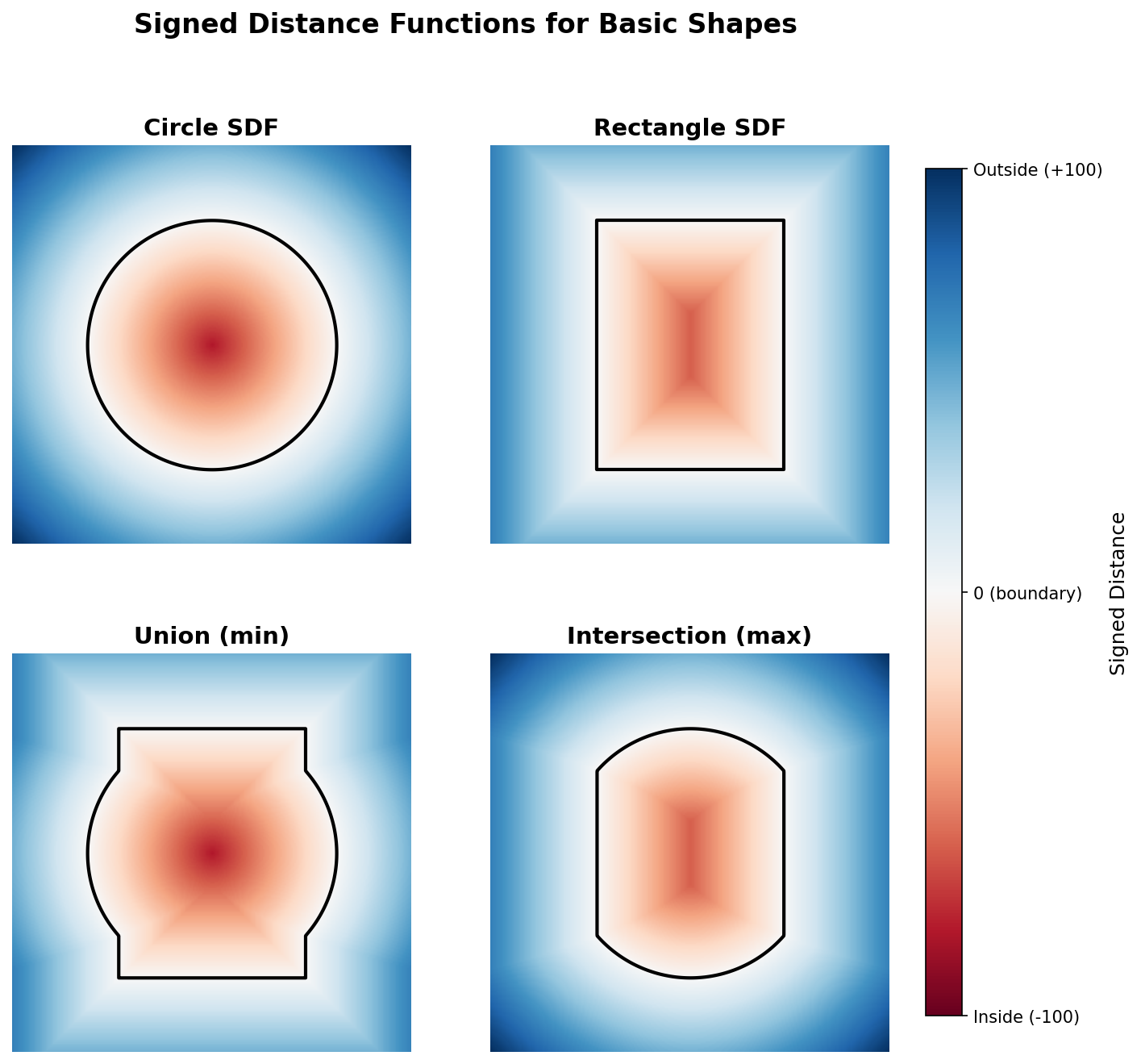
The rectangle SDF is the same idea applied per axis: np.maximum(np.abs(x) - half_w, np.abs(y) - half_h). The maximum of the two axis-aligned signed distances is itself a valid SDF, with the corner subtleties handled by the absolute value [2].
Exercises
Three exercises in Execute → Modify → Create order: visualise a distance field, vary the centre and shape, then compose multiple SDFs.
Run the distance field
Run simple_distance_field.py and inspect the output.
import numpy as np
from PIL import Image

SIZE = 512
CENTER_X, CENTER_Y = 256, 256

Y, X = np.ogrid[0:SIZE, 0:SIZE]
distance_field = np.sqrt((X - CENTER_X) ** 2 + (Y - CENTER_Y) ** 2)

normalized = (distance_field / distance_field.max() * 255).astype(np.uint8)
Image.fromarray(normalized, mode='L').save('simple_distance_field.png')

print(f"Min distance: {distance_field.min():.1f}")
print(f"Max distance: {distance_field.max():.1f}")
Reflection questions
- How do pixel brightnesses vary with distance from the centre?
- Why is the gradient circular on a square canvas?
- Where is the maximum distance, and what is its approximate value?
Answers
Pixel-to-distance — linear. The brightness at each pixel is the Euclidean distance from the centre, normalised to [0, 255]. Doubling the distance doubles the brightness (before normalisation).
Circular gradient — every level set {(x, y) : distance == d} is a circle, regardless of canvas shape. Euclidean distance is rotation-invariant. The square canvas just truncates the gradient where the circles would otherwise continue.
Maximum distance — at the corners. For a 512×512 canvas with the centre at (256, 256), the corner distance is sqrt(256² + 256²) ≈ 362 pixels.
Move it, stretch it, invert it
Edit the quick-start code to produce these three pictures.
Goals
- Off-centre — move the source point to
(50, 50)(top-left corner). - Elliptical field — stretch the gradient vertically by scaling the y-component.
- Inverted — bright at the centre, dark at the edges.
Goal 1 — what to expect
Change CENTER_X, CENTER_Y = 50, 50. The dark point moves to the top-left, and the brightest pixel is now the opposite corner at (511, 511).
Goal 2 — what to expect
Scale one component before squaring:
distance_field = np.sqrt((X - CENTER_X) ** 2 + ((Y - CENTER_Y) * 2) ** 2)Multiplying y by 2 doubles its contribution, compressing the gradient vertically. The level sets become vertical ellipses.
Goal 3 — what to expect
Subtract from 255:
normalized = 255 - (distance_field / distance_field.max() * 255).astype(np.uint8)Brightest at the centre, darkest at the corners. Equivalent to mapping 1 - normalised.
SDF composition
Build a composition with at least two SDFs and one boolean operation. Suggestion: a ring (outer circle minus inner circle) crossed by a vertical bar (a tall rectangle SDF), unioned together.
import numpy as np
from PIL import Image

SIZE = 512
CENTER = SIZE // 2

Y, X = np.ogrid[0:SIZE, 0:SIZE]
x = X - CENTER
y = Y - CENTER

# TODO 1: outer circle SDF (radius 180)
# outer = np.sqrt(x**2 + y**2) - 180

# TODO 2: inner circle SDF (radius 100)
# inner = np.sqrt(x**2 + y**2) - 100

# TODO 3: ring = outer minus inner (use np.maximum and negation)
# ring = np.maximum(outer, -inner)

# TODO 4: vertical rectangle SDF — half-width 30, half-height 200
# rect = np.maximum(np.abs(x) - 30, np.abs(y) - 200)

# TODO 5: union the ring and the rectangle (np.minimum)
# combined = np.minimum(ring, rect)

# Visualisation: clip to [-150, 150], shift to [0, 300], scale to [0, 255]
# normalized = np.clip(combined, -150, 150)
# normalized = ((normalized + 150) / 300 * 255).astype(np.uint8)
# Image.fromarray(normalized, mode='L').save('sdf_combination.png')
Hint 1 — building shape primitives
def circle(x, y, r):
    return np.sqrt(x ** 2 + y ** 2) - r

def rect(x, y, hw, hh):
    return np.maximum(np.abs(x) - hw, np.abs(y) - hh)
The rectangle SDF only computes the “outside” distance correctly — for points outside the rectangle near a corner, it underestimates the true Euclidean distance — but it is correct in sign and good enough for visualisation [2].
Hint 2 — subtraction is max-with-negation
A ring is “inside the outer circle AND outside the inner circle”:
ring = np.maximum(outer_sdf, -inner_sdf)-inner_sdf swaps inside/outside of the inner circle, then np.maximum keeps only the points that satisfy both halves.
Complete solution
import numpy as np
from PIL import Image

SIZE = 512
CENTER = SIZE // 2

Y, X = np.ogrid[0:SIZE, 0:SIZE]
x = X - CENTER
y = Y - CENTER

outer = np.sqrt(x ** 2 + y ** 2) - 180
inner = np.sqrt(x ** 2 + y ** 2) - 100
ring  = np.maximum(outer, -inner)

rect = np.maximum(np.abs(x) - 30, np.abs(y) - 200)

combined = np.minimum(ring, rect)

normalized = np.clip(combined, -150, 150)
normalized = ((normalized + 150) / 300 * 255).astype(np.uint8)
Image.fromarray(normalized, mode='L').save('sdf_combination.png')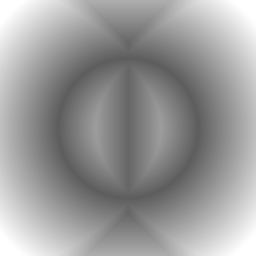
How it works:
outerandinnerare both circle SDFs with the same centre, different radii. Subtracting one from the other (viamaxand negation) gives the annular ring.rectis a rectangle SDF — taking the max of two axis-aligned signed distances yields a valid SDF for a rectangle (subject to the corner approximation noted above).np.minimum(ring, rect)unions them — every pixel takes the closer of the two boundaries.- The visualisation clips the SDF to
[-150, 150](most useful range), shifts to[0, 300], and scales to[0, 255]for grayscale.
Make it your own
- Colour map. Visualise with
matplotliband a diverging colormap:plt.imsave('out.png', combined, cmap='coolwarm'). Blue = inside, red = outside, white = boundary. - Concentric rings. Apply a sinusoid to the distance:
np.sin(distance / 20) * 127 + 128. Smaller divisors give tighter rings. - Voronoi-style. Take the minimum across multiple point SDFs:
np.minimum.reduce([sdf1, sdf2, sdf3]). Each pixel’s value is its distance to the nearest of several centres.
Downloads
simple_distance_field.py — quick start sdf_shapes.py — circle/rect/union/intersection sdf_combination_solution.py — Exercise 3 referenceSummary
Common pitfalls to avoid
- Forgetting to subtract the radius — leaves you with an unsigned distance, which is not enough for composition.
- Using
np.minimumwhere you wantednp.maximum(or vice versa) — the union/intersection swap. - Misnormalising for visualisation — distance values that go negative will wrap when cast to
uint8without clipping/shifting. - Trusting the rectangle SDF for corner cases — it underestimates distance just outside a corner. Good enough for visualisation, but not for ray-marching where precision matters.
References
- [1] Hart, J. C. (1996). Sphere tracing: A geometric method for the antialiased ray tracing of implicit surfaces. The Visual Computer, 12(10), 527–545. doi:10.1007/s003710050084
- [2] Quilez, I. (2008). Distance functions. Inigo Quilez Articles. iquilezles.org/articles/distfunctions
- [3] Green, C. (2007). Improved alpha-tested magnification for vector textures and special effects. ACM SIGGRAPH 2007 Courses, Article 9. doi:10.1145/1281500.1281665
- [4] Gonzalez, R. C., & Woods, R. E. (2018). Digital Image Processing (4th ed.). Pearson.
- [5] Harris, C. R., et al. (2020). Array programming with NumPy. Nature, 585(7825), 357–362. doi:10.1038/s41586-020-2649-2
- [6] NumPy Community. (2024). numpy.ogrid. NumPy Documentation. numpy.org
- [7] Pearson, M. (2011). Generative Art: A Practical Guide Using Processing. Manning.