2.2.1 Gradient Fields

Overview

A gradient is the simplest possible coordinate field — a function f(x, y) that turns pixel positions into brightness values. Set f(x, y) = x and you get a horizontal gradient. Set f(x, y) = y and you get a vertical one. Set f(x, y) = (x + y) / 2 and you get a diagonal. This pattern — value as a function of position — is the conceptual seed of every procedural texture you will write later in the module: spirals, vector fields, distance fields, and the noise textures of Module 06. The mechanic for turning a 1D linspace into a 2D image is two NumPy operations: np.tile (for axis-aligned gradients) and broadcasting (for everything else) [1].

Learning objectives

1. Use np.linspace to generate evenly-spaced grayscale values that interpolate between two endpoints.
2. Tile a 1D linspace into 2D with np.tile, controlling gradient direction by tiling either rows or columns.
3. Combine horizontal and vertical 1D components via NumPy broadcasting to build diagonal and radial gradients.
4. Cast back to uint8 after floating-point combinations, keeping image data in the displayable range.

Quick start — a black-to-white horizontal gradient

import numpy as np
from PIL import Image

height, width = 300, 800

# 1D linspace: 800 evenly-spaced values between 0 and 255
gradient_values = np.linspace(0, 255, width, dtype=np.uint8)

# np.tile repeats the row `height` times to fill the canvas
gradient_image = np.tile(gradient_values, (height, 1))

Image.fromarray(gradient_image, mode='L').save('simple_gradient.png')

Core concepts

Concept 1 — np.linspace as the value generator

np.linspace(start, stop, num) returns num evenly-spaced values from start to stop, inclusive at both ends. The arithmetic per element is

value[i] = start + i · (stop - start) / (num - 1).

For grayscale image data the natural range is 0 to 255, so np.linspace(0, 255, width, dtype=np.uint8) is the canonical gradient row [2]. The dtype=np.uint8 argument is not optional — Pillow stores standard 8-bit images as unsigned bytes, and passing a float64 array can produce display oddities or silent type conversion.

import numpy as np

# 5 evenly-spaced values from 0 to 100
print(np.linspace(0, 100, 5))
# → [ 0.  25.  50.  75. 100.]

# Cast to image bytes
print(np.linspace(0, 255, 5, dtype=np.uint8))
# → [ 0  63 127 191 255]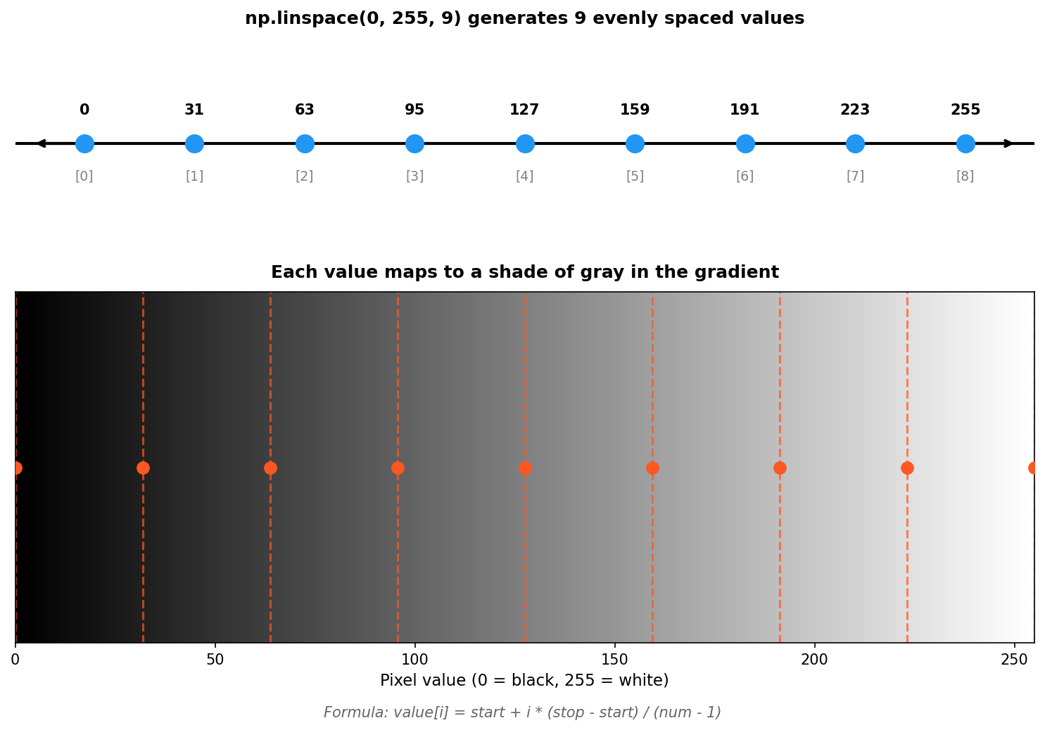

Concept 2 — Tiling and reshaping for gradient direction

np.tile(array, reps) repeats array a given number of times along each axis. The shape of reps determines the axis of repetition. For a horizontal gradient you start with a row, then tile downward; for a vertical gradient, start with a column and tile rightward [3]:

size = 200

# Horizontal: values change across columns
horizontal = np.tile(
    np.linspace(0, 255, size, dtype=np.uint8),
    (size, 1),
)

# Vertical: values change down rows
vertical = np.tile(
    np.linspace(0, 255, size, dtype=np.uint8).reshape(-1, 1),
    (1, size),
)

The reshape(-1, 1) turns a 1D (size,) array into a 2D (size, 1) column vector. The -1 tells NumPy “figure out this dimension from the array size”. After reshape, tile(..., (1, size)) clones the column across the width. The linspace direction is the same in both cases — only the axis of repetition changes.

Concept 3 — Broadcasting horizontal and vertical components

Once you have a row vector h and a column vector v, broadcasting combines them into a full 2D image without any loops. Adding shapes (size,) and (size, 1) produces a (size, size) result where element (y, x) equals h[x] + v[y] [4]:

size = 400

h = np.linspace(0, 255, size)               # shape (400,)
v = np.linspace(0, 255, size).reshape(-1, 1)  # shape (400, 1)

# Broadcast: (400,) + (400, 1) → (400, 400)
diagonal = (h + v) / 2
diagonal_image = diagonal.astype(np.uint8)

The division by 2 keeps the result in the displayable range — adding two values up to 255 each gives up to 510, which overflows uint8. Whenever you combine k linspaces, divide by k to stay safe (or np.clip if you want saturation). The final .astype(np.uint8) is necessary because (h + v) / 2 returns floats.

Exercises

Three exercises in Execute → Modify → Create order: run a horizontal gradient, change its direction and range, then combine components into a diagonal.

import numpy as np
from PIL import Image

height = 300
width = 800
gradient_values = np.linspace(0, 255, width, dtype=np.uint8)
gradient_image = np.tile(gradient_values, (height, 1))

Image.fromarray(gradient_image, mode='L').save('simple_gradient.png')

print(f"First 5 values: {gradient_values[:5]}")
print(f"Last 5 values:  {gradient_values[-5:]}")
print(f"Middle value:   {gradient_values[width // 2]}")

vertical_values = np.linspace(0, 255, height, dtype=np.uint8).reshape(-1, 1)
gradient_image = np.tile(vertical_values, (1, width))

gradient_values = np.linspace(128, 255, width, dtype=np.uint8)

# Swap the range
gradient_values = np.linspace(255, 0, width, dtype=np.uint8)

# Or reverse the array
gradient_values = np.linspace(0, 255, width, dtype=np.uint8)[::-1]

CREATE III.

Diagonal gradient via broadcasting

Build a 400×400 diagonal gradient: pure black at the top-left corner, pure white at the bottom-right, mid-gray (~127) at the centre.

python · exercise3_starter.py Copy

import numpy as np
from PIL import Image

size = 400

# TODO 1: build a horizontal 1D linspace from 0 to 255 with `size` values
# horizontal = ...

# TODO 2: build a vertical column vector with the same values
# vertical = ...

# TODO 3: combine them via broadcasting; divide by 2 to stay in [0, 255]
# diagonal = ...

# TODO 4: cast to uint8 before saving
# gradient_image = ...

Image.fromarray(gradient_image, mode='L').save('diagonal_gradient.png')

Hint 1 — the two 1D components

linspace for both, but reshape the vertical one:

horizontal = np.linspace(0, 255, size)
vertical = np.linspace(0, 255, size).reshape(-1, 1)

Notice the floats here — you will average them, then cast at the end.

Hint 2 — broadcasting and the divide

diagonal = (horizontal + vertical) / 2

The (size,) plus (size, 1) broadcast produces a (size, size) 2D array. The / 2 is what keeps the maximum at 255 instead of 510.

Hint 3 — back to uint8

After the division you have float values. Pillow needs uint8:

gradient_image = diagonal.astype(np.uint8)

This truncates rather than rounds — a single-pixel difference at most for image data, which is invisible.

Complete solution

python · exercise3_solution.py Copy

import numpy as np
from PIL import Image

size = 400

horizontal = np.linspace(0, 255, size)
vertical = np.linspace(0, 255, size).reshape(-1, 1)

diagonal = (horizontal + vertical) / 2
gradient_image = diagonal.astype(np.uint8)

Image.fromarray(gradient_image, mode='L').save('diagonal_gradient.png')

How it works:

• horizontal is a (400,) row vector; vertical is a (400, 1) column vector.
• Adding them triggers broadcasting: NumPy treats the singleton axes as “stretch me”, and the sum has shape (400, 400) with element (y, x) = horizontal[x] + vertical[y].
• The division by 2 keeps values in [0, 255]. The corners come out to 0, 127.5, 127.5, 255.
• The final cast turns floats into displayable bytes.

Make it your own

• Anti-diagonal. Swap to (horizontal + vertical[::-1, :]) / 2 (or reverse the vertical linspace) and the bright corner moves to the bottom-left.
• Radial gradient. Replace (h + v) / 2 with np.sqrt((h - 127.5)**2 + (v - 127.5)**2) for a circular falloff from the centre.
• Colour gradient. Build three different linspaces (one per channel) and stack with np.stack([r, g, b], axis=-1) for a smooth hue transition.

Downloads

Summary

Common pitfalls to avoid

• Forgetting dtype=np.uint8 and ending up with float images that Pillow misinterprets.
• Adding horizontal + vertical without dividing by 2 — values clip to 255 across the bright half of the canvas.
• Mixing up (size,) and (size, 1) shapes — broadcasting still produces a 2D array, but along the wrong axis.
• Reshaping with the wrong dimension order: .reshape(1, -1) makes a row, .reshape(-1, 1) makes a column. The minus sign tells NumPy which dimension to infer.

References

- [1] Galanter, P. (2016). Generative art theory. In C. Paul (Ed.), A Companion to Digital Art (pp. 146–180). Wiley-Blackwell. doi:10.1002/9781118475249.ch8
- [2] NumPy Community. (2024). numpy.linspace. NumPy Documentation. numpy.org
- [3] NumPy Community. (2024). numpy.tile. NumPy Documentation. numpy.org
- [4] Harris, C. R., et al. (2020). Array programming with NumPy. Nature, 585(7825), 357–362. doi:10.1038/s41586-020-2649-2
- [5] Gonzalez, R. C., & Woods, R. E. (2018). Digital Image Processing (4th ed.). Pearson.
- [6] Pearson, M. (2011). Generative Art: A Practical Guide Using Processing. Manning.
- [7] Sweller, J., van Merriënboer, J. J. G., & Paas, F. (2020). Cognitive architecture and instructional design: 20 years later. Educational Psychology Review, 31(2), 261–292.