2.2.2 Archimedean Spiral
Convert polar coordinates (angle, radius) to Cartesian pixels and trace an Archimedean spiral with `r = a + bθ`, then tune the growth rate and colour-interpolate along the curve.
Overview
The Archimedean spiral has one equation: $r = a + b\theta$. The radius grows linearly with the angle, so consecutive turns sit at a constant distance from each other [1]. Translate that single line of polar-coordinate arithmetic into pixels — convert each $(r, \theta)$ to Cartesian, draw a line to the previous point — and you have the spiral. The same template extends to logarithmic spirals (replace + with *), star-like rose curves (next module), and the entire family of polar-coordinate art that comes after.
Learning objectives
- Convert between polar
(r, θ)and Cartesian(x, y)coordinates usingcosandsin. - Implement the Archimedean spiral equation
r = a + b·θand trace it pixel-by-pixel. - Use a Python generator to model an open-ended sequence of spiral points without storing them all.
- Linearly interpolate two colours along the spiral’s progress for a gradient stroke.
Quick start — one Archimedean spiral
import numpy as np
from PIL import Image

def draw_line(canvas, x0, y0, x1, y1, color):
    n = max(abs(x1 - x0), abs(y1 - y0)) + 1
    xs = np.linspace(x0, x1, n).round().astype(int)
    ys = np.linspace(y0, y1, n).round().astype(int)
    h, w = canvas.shape[:2]
    inside = (xs >= 0) & (xs < w) & (ys >= 0) & (ys < h)
    canvas[ys[inside], xs[inside]] = color

WIDTH, HEIGHT = 512, 512
cx, cy = WIDTH // 2, HEIGHT // 2
canvas = np.zeros((HEIGHT, WIDTH, 3), dtype=np.uint8)

def spiral_points(start_radius=10, growth_rate=4.0, num_points=500):
    for i in range(num_points):
        theta = i * 0.1
        r = start_radius + growth_rate * theta
        x = int(cx + r * np.cos(theta))
        y = int(cy + r * np.sin(theta))
        yield x, y

points = spiral_points()
prev_x, prev_y = next(points)
for x, y in points:
    draw_line(canvas, prev_x, prev_y, x, y, [255, 255, 255])
    prev_x, prev_y = x, y

Image.fromarray(canvas, mode='RGB').save('simple_spiral.png')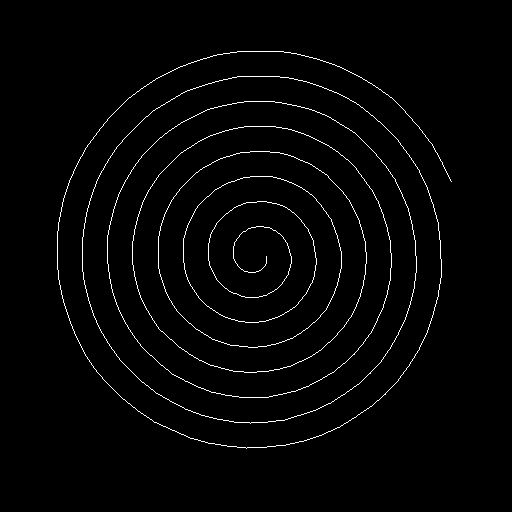
Core concepts
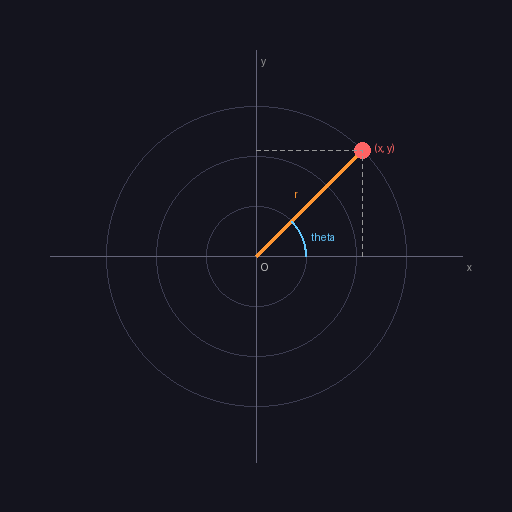
Concept 1 — Polar coordinates and the conversion
A point can be addressed two ways. In Cartesian coordinates you give horizontal and vertical offsets (x, y) from an origin. In polar coordinates you give an angle θ and a distance r, and the same point comes out:
$$x = r \cos\theta, \qquad y = r \sin\theta$$
For anything with rotational structure — circles, spirals, rose curves, sunbursts — polar is the natural language. The conversion is one line of code per coordinate [2].
Concept 2 — The Archimedean spiral
Archimedes’ spiral is the simplest polar curve where both r and θ vary:
$$r = a + b,\theta$$
with a the starting radius and b the growth rate. Each full turn of θ (one 2π increment) adds 2πb to the radius — a constant gap between successive turns. This separates it from the logarithmic spiral seen in nautilus shells, where the radius multiplies rather than adds, and the gap grows with each turn [3].
# Trace 500 points along the spiral
start_radius = 5     # 'a' — the inner radius
growth_rate = 0.5    # 'b' — radius added per radian
angle_step = 0.1     # how far to advance per point

for i in range(500):
    theta = i * angle_step
    r = start_radius + growth_rate * theta
    # convert and plot
The two parameters that decide what the spiral looks like are growth_rate (how fast it opens) and angle_step (how smoothly the curve traces — small steps give clean curves, large steps give a polygonal staircase).
Concept 3 — Python generators for open-ended sequences
A spiral is theoretically infinite — θ can keep growing forever. A Python generator function models that naturally: instead of return-ing a list, it yields one value at a time, and the caller pulls more as needed [4]:
def spiral_points(start_radius, growth_rate, num_points):
    for i in range(num_points):
        theta = i * 0.1
        r = start_radius + growth_rate * theta
        x = int(cx + r * np.cos(theta))
        y = int(cy + r * np.sin(theta))
        yield x, y      # pause here, send (x, y) back to the caller

# Consume the generator one point at a time
for x, y in spiral_points(5, 0.5, 1000):
    ...
Three reasons generators fit this kind of work: memory (no list of 1000 tuples sitting around), composability (a spiral generator chains naturally into a draw-line consumer), and a conceptual match (a spiral is an iterative process, not a fixed-size dataset).
Exercises
Three exercises in Execute → Modify → Create order: run the basic spiral, tune its parameters, then add a colour gradient along the path.
Run the Archimedean spiral
Run simple_spiral.py and observe the output.
import numpy as np
from PIL import Image

def draw_line(canvas, x0, y0, x1, y1, color):
    n = max(abs(x1 - x0), abs(y1 - y0)) + 1
    xs = np.linspace(x0, x1, n).round().astype(int)
    ys = np.linspace(y0, y1, n).round().astype(int)
    h, w = canvas.shape[:2]
    inside = (xs >= 0) & (xs < w) & (ys >= 0) & (ys < h)
    canvas[ys[inside], xs[inside]] = color

WIDTH, HEIGHT = 512, 512
cx, cy = WIDTH // 2, HEIGHT // 2
canvas = np.zeros((HEIGHT, WIDTH, 3), dtype=np.uint8)

def spiral_points(start_radius=10, growth_rate=4.0, num_points=500):
    for i in range(num_points):
        theta = i * 0.1
        r = start_radius + growth_rate * theta
        x = int(cx + r * np.cos(theta))
        y = int(cy + r * np.sin(theta))
        yield x, y

points = spiral_points()
prev_x, prev_y = next(points)
for x, y in points:
    draw_line(canvas, prev_x, prev_y, x, y, [255, 255, 255])
    prev_x, prev_y = x, y

Image.fromarray(canvas, mode='RGB').save('simple_spiral.png')
Reflection questions
- Where does the spiral start drawing — at the centre or the outer edge?
- Roughly how many full turns are visible, given
num_points=500andangle_step=0.1? - What would change visually if you swapped
np.cosandnp.sinfor the x/y assignment?
Answers
Start point — the centre. At i=0 the angle is 0 and the radius is start_radius=10, which is just 10 pixels off-centre. The spiral grows outward from there.
Number of turns — total angle is 500 · 0.1 = 50 radians. Divide by 2π ≈ 6.283 and you get about 7.96 turns. The outermost turn lives roughly at radius 10 + 4 · 50 = 210 pixels — close to the canvas edge.
Swap cos and sin — swapping cos and sin reflects the spiral about the line y = x. The shape stays the same; only the orientation changes. (This is because cos and sin are related by a phase shift of π/2.)
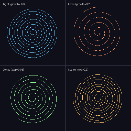
Tune the spiral parameters
Edit exercise1_execute.py to produce these three pictures.
Goals
- Tighter — more turns packed into the same canvas (smaller
growth_rate). - Looser — fewer turns, expanding faster (larger
growth_rate). - Inward — starts at the outer edge and spirals into the centre.
Goal 1 — what to expect
Drop the growth_rate and lengthen the loop:
spiral_points(start_radius=5, growth_rate=0.3, num_points=600)The spiral expands more slowly, so 600 points fit into the same canvas with more visible turns.
Goal 2 — what to expect
Raise the growth_rate and shorten the loop:
spiral_points(start_radius=5, growth_rate=1.0, num_points=300)Each turn is much wider, so the spiral reaches the edge in fewer turns.
Goal 3 — what to expect
Start with a large radius and use a negative growth rate:
spiral_points(start_radius=200, growth_rate=-0.4, num_points=500)The radius starts at 200 and shrinks toward zero; the spiral winds inward.
Colour-gradient spiral
Build a spiral whose stroke transitions from red at the centre to blue at the outer edge. Reuse the generator pattern; add a per-point progress value (0 at the start, 1 at the end) and interpolate between two RGB triples.
import numpy as np
from PIL import Image

# ... draw_line and canvas setup as before ...

start_color = np.array([255, 50, 50])    # red
end_color   = np.array([50, 50, 255])    # blue

def spiral_with_progress(start_radius, growth_rate, num_points):
    for i in range(num_points):
        # TODO 1: compute theta, r, and (x, y)
        # TODO 2: compute progress = i / (num_points - 1)
        # TODO 3: yield (x, y, progress)
        pass

def interpolate_color(c0, c1, t):
    # TODO 4: clamp t to [0, 1] and return (1-t)*c0 + t*c1 as uint8
    pass

# TODO 5: walk the generator; for each segment, compute its colour with
# interpolate_color(progress) and pass it to draw_line.

Image.fromarray(canvas, mode='RGB').save('color_spiral.png')
Hint 1 — progress in the generator
progress is just a normalised loop index:
progress = i / (num_points - 1) if num_points > 1 else 0
yield x, y, progress
Hint 2 — linear interpolation between colours
def interpolate_color(c0, c1, t):
    t = max(0.0, min(1.0, t))
    return ((1 - t) * c0 + t * c1).astype(np.uint8)
The clamp is defensive — if progress ever drifts outside [0, 1] (which can happen with custom step counts) you avoid out-of-range RGB values.
Complete solution
import numpy as np
from PIL import Image

def draw_line(canvas, x0, y0, x1, y1, color):
    n = max(abs(x1 - x0), abs(y1 - y0)) + 1
    xs = np.linspace(x0, x1, n).round().astype(int)
    ys = np.linspace(y0, y1, n).round().astype(int)
    h, w = canvas.shape[:2]
    inside = (xs >= 0) & (xs < w) & (ys >= 0) & (ys < h)
    canvas[ys[inside], xs[inside]] = color

WIDTH, HEIGHT = 512, 512
cx, cy = WIDTH // 2, HEIGHT // 2
canvas = np.zeros((HEIGHT, WIDTH, 3), dtype=np.uint8)

start_color = np.array([255, 50, 50])
end_color   = np.array([50, 50, 255])

def spiral_with_progress(start_radius, growth_rate, num_points):
    for i in range(num_points):
        theta = i * 0.1
        r = start_radius + growth_rate * theta
        x = int(cx + r * np.cos(theta))
        y = int(cy + r * np.sin(theta))
        progress = i / (num_points - 1) if num_points > 1 else 0
        yield x, y, progress

def interpolate_color(c0, c1, t):
    t = max(0.0, min(1.0, t))
    return ((1 - t) * c0 + t * c1).astype(np.uint8)

points = spiral_with_progress(5, 0.5, 500)
prev_x, prev_y, _ = next(points)
for x, y, progress in points:
    color = interpolate_color(start_color, end_color, progress)
    draw_line(canvas, prev_x, prev_y, x, y, color)
    prev_x, prev_y = x, y

Image.fromarray(canvas, mode='RGB').save('color_spiral.png')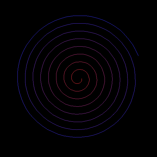
How it works:
- The generator now yields a third value,
progress, alongside(x, y). Adding a value costs nothing — generators are flexible about what they yield. interpolate_coloris plain linear interpolation:(1-t)*c0 + t*c1. Same operation as the gradient sky in 2.1.2.- Drawing per-segment with the interpolated colour produces the smooth red-to-blue transition.
Make it your own
- Logarithmic spiral. Replace
r = a + b*θwithr = a * exp(b*θ). Pick a smallb(around 0.1) — exponential growth ramps fast. - Double spiral. Run two generators with
thetashifted byπ(half a turn) and draw both onto the same canvas in different colours — the result reads like a galaxy’s arms. - Rainbow. Cycle through HSV hues with
progress, then convert back to RGB withcolorsys.hsv_to_rgbfor a six-colour rainbow.
Downloads
simple_spiral.py — quick start spiral_variations.py — parameter sweep color_spiral_solution.py — gradient strokeSummary
Common pitfalls to avoid
- Passing degrees into
np.cos/np.sin— they expect radians. Usenp.radians(deg)if you start in degrees. - Forgetting to add
cx, cyto the converted coordinates — the spiral renders in the top-left corner instead of centred. - Picking a
growth_rateso large that the second turn already exits the canvas. - Casting floats to
intwith.astype(int)after broadcasting and getting truncation gaps — usenp.round().astype(int)if a gap is visible.
References
- [1] Heath, T. L. (Ed.). (1897). The Works of Archimedes. Cambridge University Press. English edition of Archimedes’ On Spirals (c. 225 BCE).
- [2] Coolidge, J. L. (1952). The origin of polar coordinates. The American Mathematical Monthly, 59(2), 78–85. doi:10.2307/2307104
- [3] Thompson, D. W. (1917). On Growth and Form. Cambridge University Press.
- [4] Python Software Foundation. (2024). Functional Programming HOWTO — Generators. Python Documentation. docs.python.org
- [5] NumPy Community. (2024). Trigonometric functions. NumPy Documentation. numpy.org
- [6] Pearson, M. (2011). Generative Art: A Practical Guide Using Processing. Manning.
- [7] Foley, J. D., van Dam, A., Feiner, S. K., & Hughes, J. F. (1990). Computer Graphics: Principles and Practice (2nd ed.). Addison-Wesley.