2.3.2 Rose Curves

Overview

The rose curve — Guido Grandi’s rhodonea, 1723 — is a polar curve so compact that the whole flower fits in one equation:

$$r = a \cos(k\theta).$$

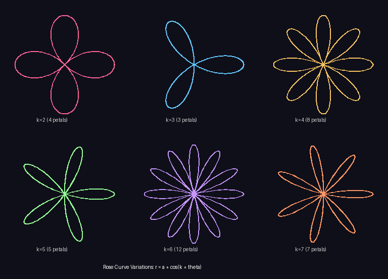
A controls the petal length; k controls everything else. The most surprising result, and the one Grandi noticed first, is the parity rule: if k is odd, the curve has exactly k petals; if k is even, it has 2k petals [1]. In this lesson you will draw rhodonea curves in NumPy using the same polar-to-Cartesian conversion from the spiral lesson, see the parity rule for yourself across a panel of k values, then colour each petal individually by mapping the angle to a palette index.

Learning objectives

1. Implement the rose-curve polar equation r = a · cos(k · θ) and trace it on a pixel canvas.
2. Predict the petal count from k using the odd/even parity rule (odd k → k petals, even k → 2k petals).
3. Convert each polar (r, θ) to Cartesian (x, y) pixel coordinates with cos/sin.
4. Colour each petal individually by mapping the current angle to a palette index.

Quick start — a 5-petal rose

import numpy as np
from PIL import Image, ImageDraw

CANVAS_SIZE = 512
CENTER = CANVAS_SIZE // 2
K = 5
AMPLITUDE = 180

image = Image.new('RGB', (CANVAS_SIZE, CANVAS_SIZE), (15, 15, 25))
draw = ImageDraw.Draw(image)

# r = a · cos(k · θ)
theta = np.linspace(0, 2 * np.pi, 1000)
r = AMPLITUDE * np.cos(K * theta)

# Polar → Cartesian
x = CENTER + r * np.cos(theta)
y = CENTER + r * np.sin(theta)

points = list(zip(x.astype(int), y.astype(int)))
draw.line(points, fill=(255, 100, 150), width=2)

image.save('simple_rose.png')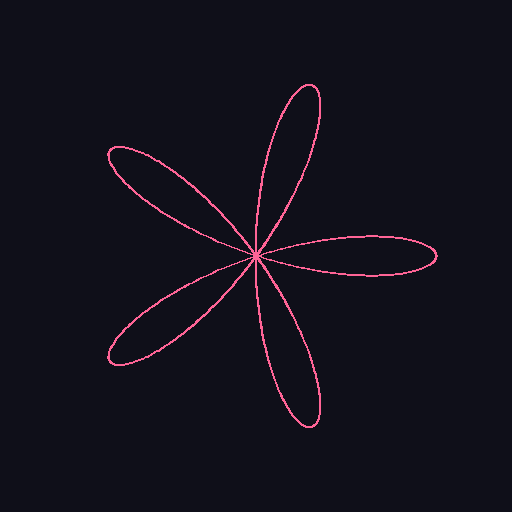

Core concepts

Concept 1 — The rose curve equation

The rose (or rhodonea) curve is the polar curve

$$r = a \cos(k\theta).$$

a is the amplitude — the petal length. k decides the petal count (next concept). To plot on a pixel canvas, the same polar-to-Cartesian transform from the spiral lesson:

$$x(\theta) = c_x + r(\theta) \cos\theta, \qquad y(\theta) = c_y + r(\theta) \sin\theta.$$

A sine version r = a sin(kθ) exists too — same shape, rotated by 90°. The mechanism is identical for both [2].

theta = np.linspace(0, 2 * np.pi, 1000)
r = amplitude * np.cos(k * theta)

x = center + r * np.cos(theta)
y = center + r * np.sin(theta)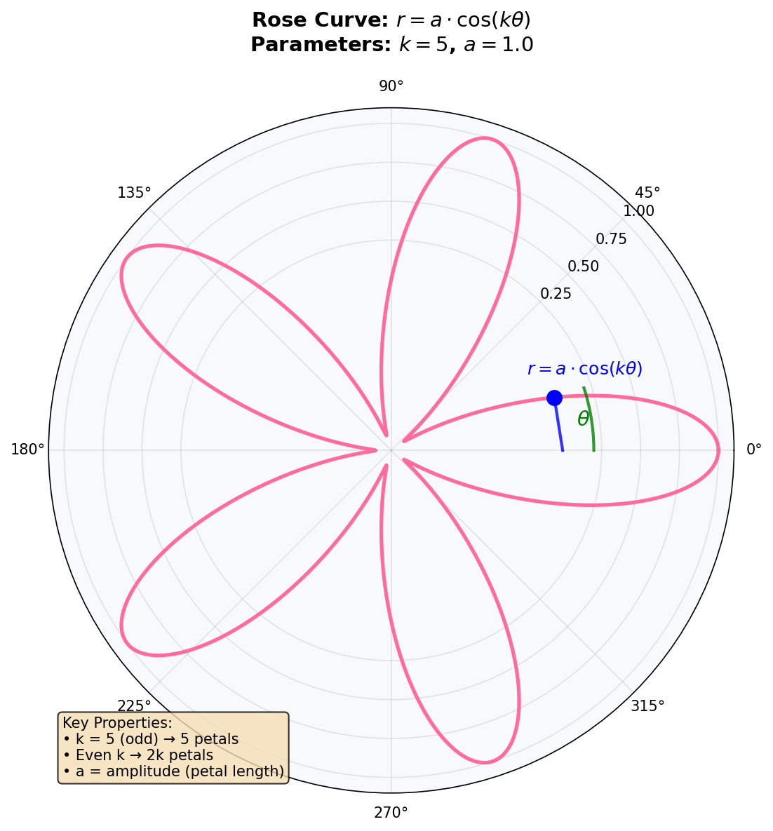

Concept 2 — The parity rule for petal counts

The strangest property of the rose: the number of petals depends on whether k is odd or even.

• Odd k — exactly k petals.
• Even k — exactly 2k petals.

Why? Look at what cos(k·θ) does as θ sweeps [0, 2π]. The argument k·θ makes k full cycles of cosine, with k positive humps and k negative humps. A positive r traces a petal in direction θ. A negative r traces a petal in the opposite direction (θ + π).

• When k is odd, each negative-r petal lands on top of an earlier positive-r petal — every petal is traced twice and you see k distinct petals.
• When k is even, positive-r and negative-r petals interleave around the circle without overlapping. You see 2k distinct petals [1, 3].

Concept 3 — Per-petal colour by angle mapping

To colour each petal independently, map the current angle θ to a petal index, then index into a palette. The angular width of one petal is π / k for the cos version with odd k (each petal is traced over half a cosine cycle), which gives:

PETAL_COLORS = [
    (255, 100, 100),  # red
    (255, 200, 100),  # orange
    (255, 255, 100),  # yellow
    (100, 255, 100),  # green
    (100, 100, 255),  # blue
]

def petal_color(theta_value, k):
    petal_index = int(theta_value * k / np.pi) % len(PETAL_COLORS)
    return PETAL_COLORS[petal_index]

The % len(PETAL_COLORS) makes the function robust if the palette has fewer entries than petals — it cycles. Drawing per-segment then becomes the standard parametric pattern: for each t, query the petal colour and draw the line segment between the previous and current (x, y).

Exercises

Three exercises in Execute → Modify → Create order: run a 5-petal rose, change the parameters to see the parity rule, then build a multi-coloured rose.

import numpy as np
from PIL import Image, ImageDraw

CANVAS_SIZE = 512
CENTER = CANVAS_SIZE // 2
K_PARAMETER = 5
AMPLITUDE = 180

image = Image.new('RGB', (CANVAS_SIZE, CANVAS_SIZE), (15, 15, 25))
draw = ImageDraw.Draw(image)

theta = np.linspace(0, 2 * np.pi, 1000)
r = AMPLITUDE * np.cos(K_PARAMETER * theta)

x = CENTER + r * np.cos(theta)
y = CENTER + r * np.sin(theta)

points = list(zip(x.astype(int), y.astype(int)))
draw.line(points, fill=(255, 100, 150), width=2)

image.save('simple_rose.png')

CREATE III.

Per-petal colours

Render a 5-petal rose with each petal in a different colour. Use a 5-entry palette and the angle-to-index helper from Concept 3.

python · exercise3_starter.py Copy

import numpy as np
from PIL import Image, ImageDraw

CANVAS_SIZE = 512
CENTER = CANVAS_SIZE // 2
K = 5
AMPLITUDE = 180

PETAL_COLORS = [
    (255, 100, 100),
    (255, 200, 100),
    (255, 255, 100),
    (100, 255, 100),
    (100, 100, 255),
]

def petal_color(theta_value, k):
    # TODO 1: return a colour from PETAL_COLORS based on the angle.
    # The petal index for cos(k·θ) is roughly int(θ · k / π) % len(PETAL_COLORS).
    return PETAL_COLORS[0]

image = Image.new('RGB', (CANVAS_SIZE, CANVAS_SIZE), (15, 15, 25))
draw = ImageDraw.Draw(image)

theta = np.linspace(0, 2 * np.pi, 1000)
r = AMPLITUDE * np.cos(K * theta)
x = (CENTER + r * np.cos(theta)).astype(int)
y = (CENTER + r * np.sin(theta)).astype(int)

# TODO 2: draw line segments between consecutive points; use petal_color
# at theta[i] (or the midpoint of theta[i-1] and theta[i]) for each.

image.save('colored_rose.png')

Hint 1 — angle to petal index

def petal_color(theta_value, k):
    petal_index = int(theta_value * k / np.pi) % len(PETAL_COLORS)
    return PETAL_COLORS[petal_index]

theta · k / π advances by 1 every time θ advances by π/k, which is roughly one petal’s worth of angle.

Hint 2 — drawing per-segment

for i in range(1, len(theta)):
    color = petal_color(theta[i], K)
    draw.line([(x[i - 1], y[i - 1]), (x[i], y[i])], fill=color, width=2)

Per-segment drawing is the cost of per-segment colour — one Pillow call per pair of adjacent points instead of one for the whole polyline.

Complete solution

python · exercise3_solution.py Copy

import numpy as np
from PIL import Image, ImageDraw

CANVAS_SIZE = 512
CENTER = CANVAS_SIZE // 2
K = 5
AMPLITUDE = 180

PETAL_COLORS = [
    (255, 100, 100), (255, 200, 100), (255, 255, 100),
    (100, 255, 100), (100, 100, 255),
]

def petal_color(theta_value, k):
    petal_index = int(theta_value * k / np.pi) % len(PETAL_COLORS)
    return PETAL_COLORS[petal_index]

image = Image.new('RGB', (CANVAS_SIZE, CANVAS_SIZE), (15, 15, 25))
draw = ImageDraw.Draw(image)

theta = np.linspace(0, 2 * np.pi, 1000)
r = AMPLITUDE * np.cos(K * theta)
x = (CENTER + r * np.cos(theta)).astype(int)
y = (CENTER + r * np.sin(theta)).astype(int)

for i in range(1, len(theta)):
    color = petal_color(theta[i], K)
    draw.line([(x[i - 1], y[i - 1]), (x[i], y[i])], fill=color, width=2)

image.save('colored_rose.png')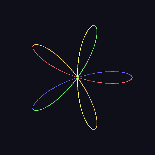

How it works:

• petal_color divides the angle range into bands of width π/k and indexes into the palette.
• The per-segment drawing loop calls draw.line once per pair of adjacent points so each segment can have its own colour.
• The modulo in int(theta * k / np.pi) % len(PETAL_COLORS) lets the palette cycle if it has fewer entries than petals.

Make it your own

• Nested roses. Draw k = 3, k = 5, k = 7 at the same centre with different amplitudes and colours.
• Gradient petals. Replace the discrete palette with a hue cycle: color = hue_to_rgb((theta[i] * k / (2 * np.pi)) % 1).
• Rose garden. Place 5 roses at scattered positions, each with a different k. The page reads as a small algorithmic floral arrangement.

Downloads

Summary

Common pitfalls to avoid

• Setting k to the desired petal count for even values — you will get twice as many petals.
• Sampling too few points — high k aliases. Bump num_points until the curve is smooth.
• Amplitude too large — petal tips clip the canvas. Keep AMPLITUDE under CANVAS_SIZE // 2 - margin.
• Forgetting the centre offset — x = r · cos(θ) (without + CENTER) renders in the top-left corner.

References

- [1] Grandi, G. (1723). Flores geometrici ex Rhodonearum, et Cloeliarum curvarum descriptione resultantes. Florence.
- [2] Lockwood, E. H. (1961). A Book of Curves. Cambridge University Press.
- [3] Weisstein, E. W. (2024). Rose. MathWorld — A Wolfram Web Resource. mathworld.wolfram.com/Rose
- [4] NumPy Community. (2024). Trigonometric functions. NumPy Documentation. numpy.org
- [5] Clark, A., et al. (2024). Pillow Documentation. pillow.readthedocs.io
- [6] Pearson, M. (2011). Generative Art: A Practical Guide Using Processing. Manning.
- [7] Foley, J. D., van Dam, A., Feiner, S. K., & Hughes, J. F. (1990). Computer Graphics: Principles and Practice (2nd ed.). Addison-Wesley.