2.1.2 Drawing Triangles

Overview

Every 3D mesh you have ever seen — from polygon-era game characters to film-quality digital doubles — is broken into triangles before the GPU touches it. The reason is geometric, not graphical: three points always define exactly one flat plane, so the rasterizer can decide which pixels belong to a triangle without ambiguity. The deciding step is called the edge function, a 1988 algorithm from Pixar that is now baked into the silicon of every modern GPU [1]. In this lesson you will implement the edge function in NumPy, contrast it with a much shorter x + x.T trick that only works for right triangles, and stack triangles into a mountain silhouette using the painter’s algorithm.

Learning objectives

1. Express a triangle as the intersection of three half-planes, each defined by an edge.
2. Implement Pineda’s edge function to rasterize an arbitrary triangle on a 2D pixel grid.
3. Recognise the x + x.T broadcasting pattern as a compact form for axis-aligned right triangles.
4. Apply the painter’s algorithm — back to front compositing — to layered triangle scenes.

Quick start — fill a triangle

import numpy as np
from PIL import Image

height, width = 400, 400
y_coords, x_coords = np.meshgrid(np.arange(height), np.arange(width), indexing='ij')

# Vertices in clockwise order
v1 = (200, 50)    # top
v2 = (350, 350)   # bottom right
v3 = (50, 350)    # bottom left

def edge(x, y, x1, y1, x2, y2):
    """Negative when (x, y) is to the right of edge (x1, y1) → (x2, y2)."""
    return (x - x1) * (y2 - y1) - (y - y1) * (x2 - x1)

e1 = edge(x_coords, y_coords, *v1, *v2) <= 0
e2 = edge(x_coords, y_coords, *v2, *v3) <= 0
e3 = edge(x_coords, y_coords, *v3, *v1) <= 0

mask = e1 & e2 & e3

canvas = np.zeros((height, width), dtype=np.uint8)
canvas[mask] = 255

Image.fromarray(canvas).save('simple_triangle.png')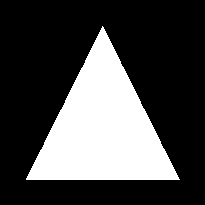

Core concepts

Concept 1 — A triangle is three half-planes intersected

Pick any line through two points $(x_1, y_1)$ and $(x_2, y_2)$. The plane on either side of that line is a half-plane. The edge function

$$E(x, y) = (x - x_1)(y_2 - y_1) - (y - y_1)(x_2 - x_1)$$

is positive on one half-plane, negative on the other, and zero exactly on the line itself [1]. It is just the 2D cross product of the edge vector and the vector from the start of the edge to the test point, so its sign tells you which way the test point lies.

A triangle is the intersection of three half-planes. If you list its vertices clockwise, inside points satisfy $E \leq 0$ for all three edges. Counterclockwise winding flips the convention to $E \geq 0$. The choice of <= (rather than strict <) is deliberate: it includes pixels exactly on the boundary, which avoids visible seams between adjacent triangles in a mesh [2].

Concept 2 — x + x.T as a broadcast trick

When the triangle is right-angled and aligned to the axes, you do not need three edge tests — only one. Build a column vector of row indices and add it to its own transpose:

import numpy as np

x = np.arange(400).reshape(400, 1)   # shape (400, 1)
distance_matrix = x + x.T             # shape (400, 400)
# element at [i, j] equals i + j

Broadcasting expands x along axis 1 and x.T along axis 0; the sum has element (i, j) = i + j. Threshold it — say i + j <= 400 — and you get a right triangle with its hypotenuse on the anti-diagonal.

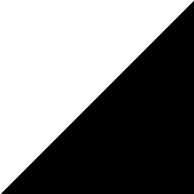
The pattern is compact and very fast, but its expressive range is narrow. The boundary is always the anti-diagonal — you cannot rotate it, you cannot place the vertices freely. For anything other than axis-aligned right triangles, fall back to the edge function. Use this trick when you actually want a right triangle; reach for edge() otherwise.

Concept 3 — Layered triangles and the painter’s algorithm

Once draw_triangle exists, composition is a question of order. To build a mountain silhouette you draw the distant mountain first, then a closer one over it, then a closer one over that. Each new triangle overwrites pixels from earlier ones, so the most recently drawn shape ends up on top. This is the painter’s algorithm — render back to front, just as a painter would lay a backdrop before foreground details [3].

For a 4-mountain landscape, sort by depth before drawing:

mountains = [
    {'peak': (400, 80),  'left': (250, 400), 'right': (500, 400), 'color': (100, 100, 120)},  # back
    {'peak': (150, 120), 'left': (0,   400), 'right': (320, 400), 'color': (70,  80,  90)},
    {'peak': (300, 180), 'left': (150, 400), 'right': (480, 400), 'color': (40,  45,  50)},
    {'peak': (80,  250), 'left': (0,   400), 'right': (200, 400), 'color': (30,  35,  40)},  # front
]
for m in mountains:
    draw_triangle(canvas, m['peak'], m['right'], m['left'], m['color'])

Reverse the iteration order and the foreground gets buried behind the background — same data, wrong result. The painter’s algorithm fails when triangles can mutually occlude each other (interlocking shapes), which is why GPUs use z-buffering for full 3D scenes. For a 2D silhouette landscape, painter’s order is exactly enough.

Exercises

Three exercises in Execute → Modify → Create order: rasterize a triangle, vary it, then layer triangles into a landscape.

import numpy as np
from PIL import Image

height, width = 400, 400
y_coords, x_coords = np.meshgrid(np.arange(height), np.arange(width), indexing='ij')

v1, v2, v3 = (200, 50), (350, 350), (50, 350)

def edge(x, y, x1, y1, x2, y2):
    return (x - x1) * (y2 - y1) - (y - y1) * (x2 - x1)

e1 = edge(x_coords, y_coords, *v1, *v2) <= 0
e2 = edge(x_coords, y_coords, *v2, *v3) <= 0
e3 = edge(x_coords, y_coords, *v3, *v1) <= 0
mask = e1 & e2 & e3

canvas = np.zeros((height, width), dtype=np.uint8)
canvas[mask] = 255
Image.fromarray(canvas).save('simple_triangle.png')

v1 = (200, 350)   # apex now at the bottom
v2 = (350, 50)    # top right
v3 = (50, 50)     # top left

v1 = (200, 150)
v2 = (250, 250)
v3 = (150, 250)

canvas = np.full((400, 400, 3), 255, dtype=np.uint8)   # white background
canvas[mask] = [255, 0, 0]                              # red triangle
Image.fromarray(canvas, mode='RGB').save('red_triangle.png')

CREATE III.

Layered mountain silhouette

Build a mountain landscape: a gradient sky and at least three overlapping mountain triangles drawn back to front.

Goal: a 500×400 RGB canvas with a vertical sky gradient (midnight blue at the top, sunset orange at the bottom) and three or more mountain triangles in front of it.

python · exercise3_starter.py Copy

import numpy as np
from PIL import Image

def draw_filled_triangle(canvas, v1, v2, v3, color):
    """Fill the triangle (v1, v2, v3) with `color` on an RGB canvas."""
    # TODO 1: build x, y coordinate grids with np.meshgrid
    # TODO 2: define an edge() helper and compute the three edge tests
    # TODO 3: combine with & into a mask, then assign color where the mask is True
    pass

def create_gradient_sky(height, width):
    """Vertical gradient from midnight blue (top) to sunset orange (bottom)."""
    sky = np.zeros((height, width, 3), dtype=np.uint8)
    # TODO 4: interpolate per-row between top and bottom colours, write into sky[y, :]
    return sky

height, width = 400, 500
canvas = create_gradient_sky(height, width)

# TODO 5: define at least 3 mountains as dicts with peak/left/right/color,
# then draw them back to front by calling draw_filled_triangle for each.

Image.fromarray(canvas).save('triangle_mountain.png')

Hint 1 — generalise the edge function

The same edge() helper from the quick start, parameterised by canvas size:

def draw_filled_triangle(canvas, v1, v2, v3, color):
    h, w = canvas.shape[:2]
    y_coords, x_coords = np.meshgrid(np.arange(h), np.arange(w), indexing='ij')
    def edge(x, y, x1, y1, x2, y2):
        return (x - x1) * (y2 - y1) - (y - y1) * (x2 - x1)
    e1 = edge(x_coords, y_coords, *v1, *v2) <= 0
    e2 = edge(x_coords, y_coords, *v2, *v3) <= 0
    e3 = edge(x_coords, y_coords, *v3, *v1) <= 0
    canvas[e1 & e2 & e3] = color

Hint 2 — the gradient sky

Linear interpolation between two RGB triples, one row at a time:

def create_gradient_sky(h, w):
    sky = np.zeros((h, w, 3), dtype=np.uint8)
    top = np.array([25, 25, 112])
    bot = np.array([255, 140, 50])
    for y in range(h):
        t = y / h
        sky[y, :] = ((1 - t) * top + t * bot).astype(np.uint8)
    return sky

You can also do this vectorised with np.linspace, but the loop is easy to read.

Hint 3 — draw order matters

Sort your mountain list so the furthest mountain is first and the closest is last. Iterate in that order, calling draw_filled_triangle per entry. Reversing the list moves the foreground behind the background, which gives the painter’s algorithm away the instant you see it.

Complete solution

python · exercise3_solution.py Copy

import numpy as np
from PIL import Image

def draw_filled_triangle(canvas, v1, v2, v3, color):
    h, w = canvas.shape[:2]
    y_coords, x_coords = np.meshgrid(np.arange(h), np.arange(w), indexing='ij')

    def edge(x, y, x1, y1, x2, y2):
        return (x - x1) * (y2 - y1) - (y - y1) * (x2 - x1)

    e1 = edge(x_coords, y_coords, *v1, *v2) <= 0
    e2 = edge(x_coords, y_coords, *v2, *v3) <= 0
    e3 = edge(x_coords, y_coords, *v3, *v1) <= 0
    canvas[e1 & e2 & e3] = color

def create_gradient_sky(h, w):
    sky = np.zeros((h, w, 3), dtype=np.uint8)
    top = np.array([25, 25, 112])
    bot = np.array([255, 140, 50])
    for y in range(h):
        t = y / h
        sky[y, :] = ((1 - t) * top + t * bot).astype(np.uint8)
    return sky

h, w = 400, 500
canvas = create_gradient_sky(h, w)

mountains = [
    {'peak': (400,  80), 'left': (250, 400), 'right': (500, 400), 'color': (100, 100, 120)},
    {'peak': (150, 120), 'left': (0,   400), 'right': (320, 400), 'color': (70,  80,  90)},
    {'peak': (300, 180), 'left': (150, 400), 'right': (480, 400), 'color': (40,  45,  50)},
    {'peak': (80,  250), 'left': (0,   400), 'right': (200, 400), 'color': (30,  35,  40)},
]
for m in mountains:
    draw_filled_triangle(canvas, m['peak'], m['right'], m['left'], m['color'])

Image.fromarray(canvas).save('triangle_mountain.png')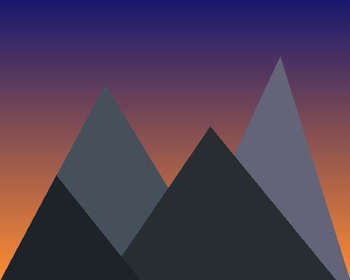

How it works:

• draw_filled_triangle rasterises a triangle by running three edge tests over the full coordinate grid and assigning the fill colour where all three pass.
• create_gradient_sky produces the backdrop with a per-row linear interpolation between two RGB triples.
• The mountain list is sorted back to front; iterating in that order means each subsequent triangle paints over what came before.

Make it your own

• Add a circular sun by computing (x - cx)**2 + (y - cy)**2 < r**2 and assigning a colour where the mask is true.
• Reflect each mountain below a “water line” with a darker, more saturated colour for a lake-foreground composition.
• Animate by sweeping the sky gradient: regenerate the canvas with shifted top/bot colours and save a sequence of frames.

Downloads

Summary

Common pitfalls to avoid

• Inconsistent winding order across triangles — keep them all clockwise (or all counterclockwise) so a single <= test works for every triangle.
• Forgetting Image.fromarray(canvas, mode='RGB') on colour canvases — Pillow can otherwise misinterpret a (H, W, 3) array.
• Drawing the foreground first — closer mountains end up behind distant ones.
• Float vertices feeding the edge function — fine numerically, but rounded pixel boundaries can drift; use integer vertices when you want pixel-exact silhouettes.

References

- [1] Pineda, J. (1988). A parallel algorithm for polygon rasterization. ACM SIGGRAPH Computer Graphics, 22(4), 17–20. doi:10.1145/378456.378457
- [2] Shirley, P., & Marschner, S. (2009). Fundamentals of Computer Graphics (3rd ed.). A K Peters/CRC Press.
- [3] Foley, J. D., van Dam, A., Feiner, S. K., & Hughes, J. F. (1990). Computer Graphics: Principles and Practice (2nd ed.). Addison-Wesley.
- [4] Gonzalez, R. C., & Woods, R. E. (2018). Digital Image Processing (4th ed.). Pearson.
- [5] Harris, C. R., et al. (2020). Array programming with NumPy. Nature, 585(7825), 357–362. doi:10.1038/s41586-020-2649-2
- [6] NumPy Community. (2024). Broadcasting. NumPy Documentation. numpy.org
- [7] Clark, A., et al. (2024). Pillow Documentation. pillow.readthedocs.io