3.1.2 Affine Transformations

Overview

Rotation was one library call. The full set of geometric transformations that preserve straight lines and parallelism — affine transformations — is four building blocks: translate, scale, rotate, shear. The trick that makes them practical is a notational sleight of hand: a 2D point gets a phantom third coordinate set to 1, and all four operations collapse into a single 3×3 matrix multiplication. Once that is true, composing transformations is just multiplying matrices, and a spiral of 24 squares becomes a single loop with one combined matrix per step [1]. This lesson is the foundation for every geometric transformation in the rest of the module.

Learning objectives

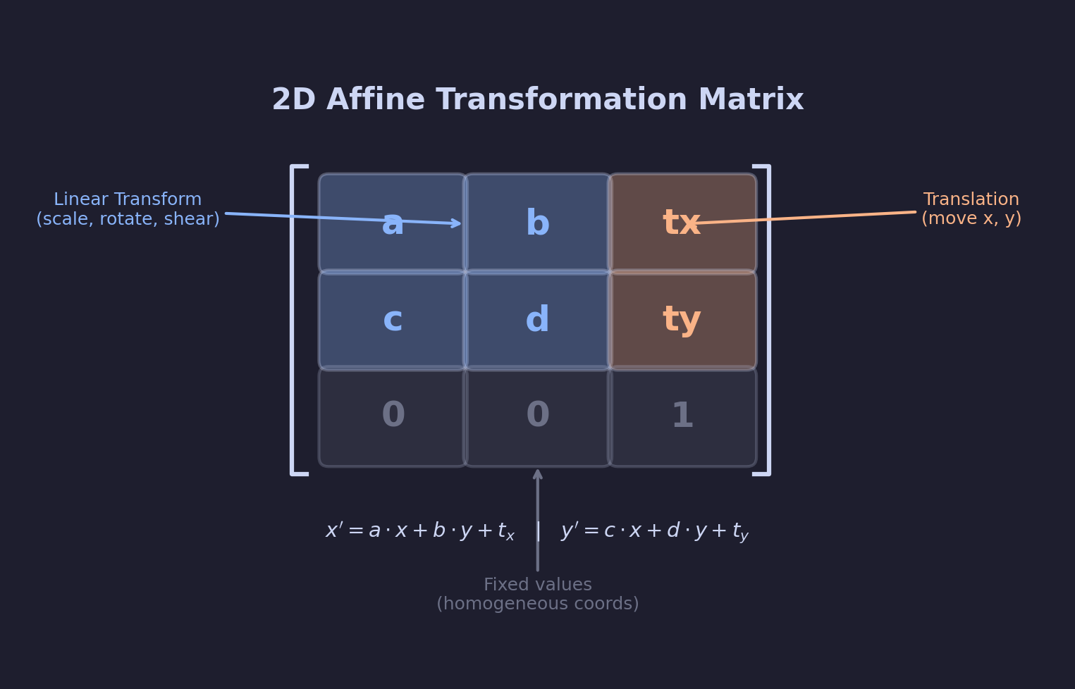
1. Read the structure of a 3×3 affine matrix: a 2×2 linear block on the top-left, a translation column on the right, and [0, 0, 1] along the bottom.
2. Build the four basic transformation matrices — translate, scale, rotate, shear — and apply them to a NumPy array of points.
3. Compose transformations with @ and predict the result by reading the chain right-to-left.
4. Use a composed matrix in a loop to draw a 24-square spiral from a single base square.

Quick start — scale and translate one square

import numpy as np
from PIL import Image, ImageDraw

canvas = np.zeros((400, 400, 3), dtype=np.uint8) + np.array([30, 30, 40], dtype=np.uint8)

square = np.array(
    [[-50, -50], [50, -50], [50, 50], [-50, 50]],
    dtype=np.float64,
)

# 2×3 affine: scale by 1.5, translate (+200, 0)
affine = np.array([
    [1.5, 0.0, 200.0],
    [0.0, 1.5,   0.0],
])

ones = np.ones((square.shape[0], 1))
homogeneous = np.hstack([square, ones])           # shape (4, 3)
transformed = (affine @ homogeneous.T).T          # shape (4, 2)

# Place both squares on the canvas
left  = (square      + np.array([100, 200])).astype(int)
right = (transformed + np.array([100, 200])).astype(int)

img = Image.fromarray(canvas)
draw = ImageDraw.Draw(img)
draw.polygon([tuple(p) for p in left],  fill=(70, 130, 200))
draw.polygon([tuple(p) for p in right], fill=(230, 150, 50))
img.save('simple_affine.png')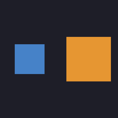

Core concepts

Concept 1 — The 3×3 matrix and homogeneous coordinates

An affine transformation is anything that preserves straight lines and parallelism. That excludes perspective (which bends parallel lines toward a vanishing point) but includes every transformation in this lesson [1]. The general form is a 3×3 matrix acting on a homogeneous column vector:

| x' |   | a  b  tx | | x |
| y' | = | c  d  ty | | y |
| 1  |   | 0  0   1 | | 1 |

The top-left 2×2 block [[a, b], [c, d]] handles every linear part — scale, rotation, shear. The right column (tx, ty) handles translation. The bottom row stays [0, 0, 1] forever; the day it changes, you are doing perspective projection instead of affine [2].

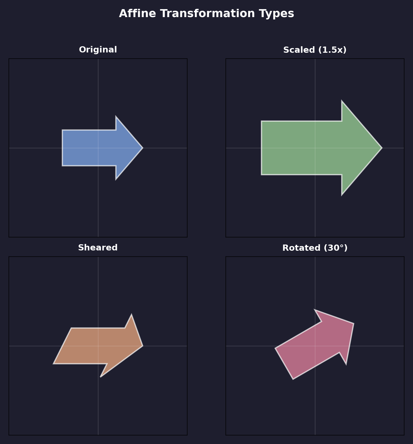
Concept 2 — The four building blocks

Every affine transformation is some product of four primitives.

import numpy as np

def translate(tx, ty):
    return np.array([[1, 0, tx], [0, 1, ty], [0, 0, 1]], dtype=np.float64)

def scale(sx, sy=None):
    if sy is None: sy = sx
    return np.array([[sx, 0, 0], [0, sy, 0], [0, 0, 1]], dtype=np.float64)

def rotate(angle_deg):
    t = np.radians(angle_deg)
    c, s = np.cos(t), np.sin(t)
    return np.array([[c, -s, 0], [s, c, 0], [0, 0, 1]], dtype=np.float64)

def shear(kx, ky=0):
    return np.array([[1, kx, 0], [ky, 1, 0], [0, 0, 1]], dtype=np.float64)

• Translate offsets every point by (tx, ty). It is the only one of the four that needs the homogeneous trick — it cannot be expressed as a 2×2 matrix [2].
• Scale multiplies coordinates by sx, sy. Equal factors give uniform scaling; unequal factors stretch and squash.
• Rotate spins around the origin using the same matrix as 3.1.1.
• Shear adds a fraction of one axis to the other. A square becomes a parallelogram.

Concept 3 — Composition with @, right-to-left

Matrix multiplication is associative but not commutative: A @ B and B @ A are usually different matrices. The order in which you multiply is the order in which transformations apply, reading right to left — the rightmost matrix touches the point first [4].

# Apply: rotation first, then scale, then translation
combined = translate(100, 50) @ scale(1.5) @ rotate(30)

# One matrix to transform any number of points
points = np.array([[0, 0], [100, 0], [100, 100], [0, 100]], dtype=np.float64)
homo = np.hstack([points, np.ones((4, 1))])
out = (combined @ homo.T).T[:, :2]

Swapping translate(100, 50) and rotate(30) gives a different output — translating first puts the corner of the square at (100, 50), then rotating spins the result around the origin, dragging the square along an arc. Rotating first spins the square in place, then translates the (already rotated) square to (100, 50). The matrix algebra captures this exactly: R @ T and T @ R are not the same matrix [1].

Exercises

Three exercises in Execute → Modify → Create order: run a simple comparison, swap matrix values to match a goal, then build a 24-square spiral.

transform = np.array([
    [0.5, 0.0, 0.0],
    [0.0, 0.5, 0.0],
])

transform = np.array([
    [1.0, 0.5, 0.0],   # x' = x + 0.5*y
    [0.0, 1.0, 0.0],
])

t = np.radians(45)
transform = np.array([
    [np.cos(t), -np.sin(t), 0.0],
    [np.sin(t),  np.cos(t), 0.0],
])

CREATE III.

A 24-square spiral

Build a spiral of 24 squares. Each square should be (a) rotated slightly more than the last, (b) scaled slightly smaller, and (c) translated to a point along an outward-spiralling polar trajectory.

python · exercise3_starter.py Copy

import numpy as np
from PIL import Image, ImageDraw

def translate(tx, ty):
    return np.array([[1, 0, tx], [0, 1, ty], [0, 0, 1]], dtype=np.float64)

def scale(s):
    return np.array([[s, 0, 0], [0, s, 0], [0, 0, 1]], dtype=np.float64)

def rotate(deg):
    t = np.radians(deg); c, s = np.cos(t), np.sin(t)
    return np.array([[c, -s, 0], [s, c, 0], [0, 0, 1]], dtype=np.float64)

def apply(points, m):
    homo = np.hstack([points, np.ones((len(points), 1))])
    return (m @ homo.T).T[:, :2]

SIZE = 500; CENTER = SIZE // 2
canvas = np.zeros((SIZE, SIZE, 3), dtype=np.uint8) + 20
img = Image.fromarray(canvas); draw = ImageDraw.Draw(img)

base = np.array([[-15, -15], [15, -15], [15, 15], [-15, 15]], dtype=np.float64)

for i in range(24):
    # TODO 1: derive angle, shrink factor, and outward distance from i.
    # angle = ...; shrink = ...; distance = ...

    # TODO 2: target position along a spiral (polar → cartesian).
    # tx = CENTER + distance * cos(2 * angle in radians)
    # ty = CENTER + distance * sin(2 * angle in radians)

    # TODO 3: compose the matrix and apply it to base.
    # combined = translate(tx, ty) @ scale(shrink) @ rotate(angle)

    # TODO 4: pick a colour from a blue → orange gradient and draw the polygon.

img.save('spiral.png')

Hint 1 — the spiral parameters

A simple linear progression works:

angle    = i * 15           # 15° more rotation per step
shrink   = max(1.0 - 0.025 * i, 0.3)   # gradually smaller, floor at 0.3
distance = 50 + 6 * i        # gradually outward

The max(..., 0.3) floor keeps the last few squares visible. Without it they collapse to a single pixel.

Hint 2 — the polar target

spiral_angle = np.radians(2 * angle)
tx = CENTER + distance * np.cos(spiral_angle)
ty = CENTER + distance * np.sin(spiral_angle)

2 * angle makes the spiral wind twice as fast as the per-square rotation, which gives the cleanest visual.

Hint 3 — colour gradient

t = i / 23
color = (int(70 + 180 * t), int(130 - 50 * t), int(200 - 150 * t))

t = 0 → blue (70, 130, 200); t = 1 → orange (250, 80, 50). Linear interp between two RGB triples — same approach as 2.1.2’s mountain sky.

Complete solution

python · exercise3_solution.py Copy

import numpy as np
from PIL import Image, ImageDraw

def translate(tx, ty):
    return np.array([[1, 0, tx], [0, 1, ty], [0, 0, 1]], dtype=np.float64)
def scale(s):
    return np.array([[s, 0, 0], [0, s, 0], [0, 0, 1]], dtype=np.float64)
def rotate(deg):
    t = np.radians(deg); c, s = np.cos(t), np.sin(t)
    return np.array([[c, -s, 0], [s, c, 0], [0, 0, 1]], dtype=np.float64)
def apply(points, m):
    homo = np.hstack([points, np.ones((len(points), 1))])
    return (m @ homo.T).T[:, :2]

SIZE = 500; CENTER = SIZE // 2
canvas = np.zeros((SIZE, SIZE, 3), dtype=np.uint8) + 20
img = Image.fromarray(canvas); draw = ImageDraw.Draw(img)

base = np.array([[-15, -15], [15, -15], [15, 15], [-15, 15]], dtype=np.float64)

for i in range(24):
    angle    = i * 15
    shrink   = max(1.0 - 0.025 * i, 0.3)
    distance = 50 + 6 * i

    spiral = np.radians(2 * angle)
    tx = CENTER + distance * np.cos(spiral)
    ty = CENTER + distance * np.sin(spiral)

    combined = translate(tx, ty) @ scale(shrink) @ rotate(angle)
    pts = apply(base, combined).astype(int)

    t = i / 23
    color = (int(70 + 180 * t), int(130 - 50 * t), int(200 - 150 * t))
    draw.polygon([tuple(p) for p in pts], fill=color, outline=(255, 255, 255))

img.save('spiral.png')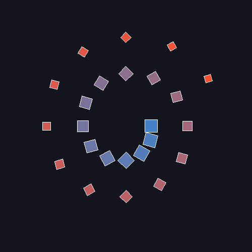

How it works:

• translate @ scale @ rotate means: rotate the base square in place around the origin, scale it down, then translate it to its target.
• The spiral shape comes from the polar (distance, spiral_angle) parametrisation of tx, ty — affine matrices on their own do not draw curves; they place a shape on a curve.
• The colour gradient is independent of the matrix work — it is a function of i / 23 and would look identical with any transformation chain.

Make it your own

• Swap base for a triangle or a pentagon. The pipeline does not care about the shape; it transforms 2D points.
• Change rotate(angle) to rotate(-angle) and watch the spiral wind the other way.
• Reverse the multiplication order: rotate(angle) @ scale(shrink) @ translate(tx, ty). The first square stays in place; subsequent squares orbit the origin instead of spiralling out.

Downloads

Summary

Common pitfalls to avoid

• Forgetting the homogeneous 1 — points have to be (x, y, 1) for translation to take effect.
• Reading the matrix chain left-to-right; the rightmost matrix applies first.
• Building matrices with np.array([[1, 0, tx], ...]) where tx is an int — NumPy infers an integer dtype and silently truncates sub-pixel translations. Use dtype=np.float64 or write 1.0 everywhere.
• Scaling around a non-origin pivot without translating first; the shape will drift instead of staying put.
• Trying to invert an affine by transposing the 3×3. The transpose works for rotation matrices, but scaling and translation need a proper np.linalg.inv.

References

- [1] Foley, J. D., van Dam, A., Feiner, S. K., & Hughes, J. F. (1995). Computer Graphics: Principles and Practice (2nd ed.). Addison-Wesley.
- [2] Hearn, D., & Baker, M. P. (2011). Computer Graphics with OpenGL (4th ed.). Pearson.
- [3] Shirley, P., & Marschner, S. (2015). Fundamentals of Computer Graphics (4th ed.). CRC Press.
- [4] Gonzalez, R. C., & Woods, R. E. (2018). Digital Image Processing (4th ed.). Pearson.
- [5] Rogers, D. F., & Adams, J. A. (1990). Mathematical Elements for Computer Graphics (2nd ed.). McGraw-Hill.
- [6] Harris, C. R., Millman, K. J., van der Walt, S. J., et al. (2020). Array programming with NumPy. Nature, 585, 357–362. doi:10.1038/s41586-020-2649-2