3.4.4 Fourier Art
Round-trip an image through `np.fft.fft2`, manipulate the frequency-domain magnitude with circular masks, and inverse-transform back. Low-pass blurs, high-pass extracts edges, glitch holes corrupt for art's sake.
Overview
A Fourier transform expresses an image as a sum of sinusoidal waves at different frequencies — Joseph Fourier’s 1822 idea, generalised by Cooley and Tukey’s 1965 FFT algorithm into the workhorse computation of modern signal processing [1, 2]. The 2D FFT of an image lives in the frequency domain: low frequencies near the centre (smooth gradients, overall brightness), high frequencies near the edges (sharp transitions, fine details). Filter the frequency representation with a circular mask, inverse-transform, and you have a blur, edge map, band-pass, or glitch artefact — all with the same three-step pipeline. The same machinery underlies JPEG compression, the optical-flow stage of every video codec, and the Fourier-feature layers showing up in modern neural networks [3].
Learning objectives
- Move an image to the frequency domain with
np.fft.fft2and centre the zero-frequency component withnp.fft.fftshift. - Visualise the magnitude spectrum with log scaling (
np.log1p). - Build circular low-pass, high-pass, and band-pass masks; apply by element-wise multiplication.
- Inverse-transform with
np.fft.ifftshiftthennp.fft.ifft2, taking the real part to get a usable image.
Quick start — FFT of a checkerboard
import numpy as np
from PIL import Image

SIZE = 256
TILE = 16

# Procedural checkerboard
rows = (np.arange(SIZE) // TILE)[:, None]
cols = (np.arange(SIZE) // TILE)[None, :]
image = np.where((rows + cols) % 2 == 0, 255.0, 0.0)

# Forward FFT, centre the zero-frequency
F = np.fft.fft2(image)
F_shift = np.fft.fftshift(F)

# Log-scaled magnitude spectrum for display
mag = np.log1p(np.abs(F_shift))
mag = (mag / mag.max() * 255).astype(np.uint8)

# Side-by-side: image | spectrum
combo = np.hstack([image.astype(np.uint8), mag])
Image.fromarray(combo, 'L').save('simple_fft_output.png')
Core concepts
Concept 1 — The frequency domain
A 2D FFT decomposes an image into a sum of complex sinusoids at every spatial frequency. For an (H, W) input, np.fft.fft2 returns an (H, W) complex array where:
F[0, 0]is the DC component — the mean brightness, scaled byH × W.F[fy, fx]for smallfy, fxcarries the low-frequency content (slow gradients).- Higher
|fy|, |fx|carries the high-frequency content (sharp edges, fine textures).
Raw FFT output puts F[0, 0] in the top-left corner. To get the centred spectrum view — where DC sits at the middle and high frequencies radiate outward — apply np.fft.fftshift:
F_shift = np.fft.fftshift(F) # DC moves from (0, 0) to (H/2, W/2)Each pixel of F_shift is a complex number; the magnitude |F_shift| describes how much energy is at that frequency, and the phase angle(F_shift) describes the spatial alignment of that frequency. Magnitude dominates appearance; phase encodes where the features are [3].
Concept 2 — Circular filters in the frequency domain
Filtering in the frequency domain is one multiplication: build a 2D mask the same shape as the FFT, multiply, inverse-transform.
Low-pass — keep frequencies inside a central disc, drop the rest:
y, x = np.indices((H, W))
cx, cy = W // 2, H // 2
dist_sq = (x - cx) ** 2 + (y - cy) ** 2
low_pass = (dist_sq <= radius ** 2).astype(np.float64)
Multiplied into the spectrum, the high frequencies vanish; sharp edges become soft because the energy that defined them is gone. The result is a blur, smoother than convolution because the cutoff is exact in frequency, not approximate.
High-pass — invert the mask:
high_pass = (dist_sq > radius ** 2).astype(np.float64)The DC and low frequencies are zeroed; only edges and textures remain. The result is an edge image — different from Sobel because it captures all frequencies above a threshold, not just first-derivative responses.
Band-pass — keep an annulus between two radii:
band_pass = ((dist_sq > r_inner ** 2) & (dist_sq <= r_outer ** 2)).astype(np.float64)Drops both the DC and the noise tail; keeps the mid-frequency “texture” band [4].
Concept 3 — The round-trip pipeline
The complete forward-filter-inverse pipeline is five lines:
F        = np.fft.fft2(image)
F_shift  = np.fft.fftshift(F)
F_filt   = F_shift * mask
F_un     = np.fft.ifftshift(F_filt)
result   = np.real(np.fft.ifft2(F_un))
Notes on the inverse pass:
ifftshiftun-does thefftshift(moves DC back to the corner). Always pair them.ifft2returns complex numbers because of floating-point rounding even though the input was real. Takenp.real; tiny imaginary components are numerical noise [5].- Clip the result to
[0, 255]before saving, especially after a high-pass filter — the result can include negative values from the lost DC.
Exercises
Three exercises in Execute → Modify → Create order: visualise the spectrum, try three filters, then build glitch art.
Visualise the spectrum
Run simple_fft.py from the downloads. Look at the spectrum next to the checkerboard.
Reflection questions
- Why are there distinct dots in the spectrum rather than a smooth distribution?
- What would happen to the spectrum if
TILEdropped from 16 to 8? - Why is the centre of the spectrum the brightest pixel?
Answers
Discrete dots — a periodic pattern decomposes into discrete frequency harmonics. The fundamental frequency of the checkerboard is one cycle per 32 pixels (32 = 2 × TILE); the dots are at the fundamental and its multiples. A non-periodic image would give a smoother spectrum.
TILE = 8 — the fundamental frequency doubles (one cycle per 16 pixels instead of 32). The dot lattice spreads twice as far from the centre; the high-frequency dots move further out toward the spectrum’s edges.
Bright centre — that is the DC component, equal to H × W × mean(image). The checkerboard is half-bright on average, so DC ≈ 256 × 256 × 127.5, dwarfing every other frequency. The log scaling makes the off-centre dots visible at all.
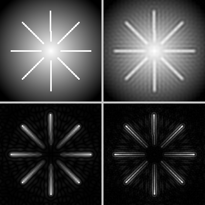
Three filter radii
Edit frequency_filter.py so it applies these three filter configurations to the same input.
Goals
- Strong blur —
radius = 15low-pass mask. - Subtle blur —
radius = 50low-pass mask. - Band-pass — keep frequencies between radii 20 and 60.
Goal 1 — what to expect
mask = (dist_sq <= 15 ** 2).astype(np.float64)A very tight disc — most frequencies removed. The output is heavily blurred; only the overall brightness gradient survives.
Goal 2 — what to expect
mask = (dist_sq <= 50 ** 2).astype(np.float64)A larger disc — most low and mid frequencies retained, only the highest dropped. The output is mildly soft, like an out-of-focus photograph.
Goal 3 — what to expect
mask = ((dist_sq > 20 ** 2) & (dist_sq <= 60 ** 2)).astype(np.float64)A ring keeping only mid-frequencies. The overall brightness (DC) is gone, so the output looks dark and grey; the fine grain is also dropped, so the picture reads as mid-scale texture. Best on natural photos with a rich mid-frequency band [4].
Glitch art with frequency holes
Build a glitch-art effect: take a photo’s FFT, multiply by an asymmetric mask (low-pass on the left half, high-pass on the right half), then poke 5 rectangular holes (“zeroed regions”) at random positions. Inverse-transform and display side-by-side with the original.
import numpy as np
from PIL import Image

img = np.array(Image.open('bbtor.jpg').convert('L'), dtype=np.float64)
H, W = img.shape

F = np.fft.fft2(img)
F_shift = np.fft.fftshift(F)

# TODO 1: build an asymmetric mask — different rule for x < W/2 vs x >= W/2.

# TODO 2: poke 5 random rectangular "glitch holes" by zeroing regions of the mask.
rng = np.random.default_rng(0)

# TODO 3: apply, inverse-transform, take real part, clip, save side-by-side.

Image.fromarray(np.hstack([img, glitched]).astype(np.uint8), 'L').save('glitch.png')
Hint 1 — asymmetric mask
y, x = np.indices((H, W))
cx, cy = W // 2, H // 2
dist_sq = (x - cx) ** 2 + (y - cy) ** 2

mask = np.zeros((H, W), dtype=np.float64)
mask[x < cx] = (dist_sq <= 40 ** 2)[x < cx]       # left half: low-pass
mask[x >= cx] = (dist_sq > 40 ** 2)[x >= cx]      # right half: high-pass
The mask is 1 inside the disc on the left and 1 outside the disc on the right. The two halves merge at the vertical centreline.
Hint 2 — random rectangular holes
for _ in range(5):
    y0 = rng.integers(0, H - 20)
    x0 = rng.integers(0, W - 20)
    h  = rng.integers(5, 20)
    w  = rng.integers(5, 20)
    mask[y0:y0 + h, x0:x0 + w] = 0
Each hole zeros a small region of the mask. The corresponding frequencies are erased; inverse-transformed, they show up as banded artifacts in the spatial domain.
Hint 3 — round-trip
F_filt = F_shift * mask
result = np.real(np.fft.ifft2(np.fft.ifftshift(F_filt)))
glitched = np.clip(result, 0, 255).astype(np.uint8)
The clip is essential — high-pass output has negative pixels because DC was removed.
Complete solution
import numpy as np
from PIL import Image

img = np.array(Image.open('bbtor.jpg').convert('L'), dtype=np.float64)
H, W = img.shape

F = np.fft.fft2(img)
F_shift = np.fft.fftshift(F)

y, x = np.indices((H, W))
cx, cy = W // 2, H // 2
dist_sq = (x - cx) ** 2 + (y - cy) ** 2

mask = np.zeros((H, W), dtype=np.float64)
left  = x <  cx
right = x >= cx
mask[left]  = (dist_sq <= 40 ** 2)[left]
mask[right] = (dist_sq >  40 ** 2)[right]

rng = np.random.default_rng(0)
for _ in range(5):
    y0 = rng.integers(0, H - 20); x0 = rng.integers(0, W - 20)
    h  = rng.integers(5, 20);     w  = rng.integers(5, 20)
    mask[y0:y0 + h, x0:x0 + w] = 0

F_filt = F_shift * mask
result = np.real(np.fft.ifft2(np.fft.ifftshift(F_filt)))
glitched = np.clip(result, 0, 255).astype(np.uint8)

side_by_side = np.hstack([img.astype(np.uint8), glitched])
Image.fromarray(side_by_side, 'L').save('glitch.png')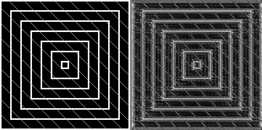
How it works:
- The mask is a boolean union: low-pass on the left, high-pass on the right. The two halves use opposite filtering rules around the same disc.
- Each random hole removes a contiguous range of frequencies. Spatially, that translates to banded or striped artifacts — the inverse FFT of a rectangular hole is a sinc-like wave [3].
- Take the real part of the inverse FFT; round-trip rounding produces tiny imaginary components that should be discarded.
Make it your own
- Scramble the phase instead of zeroing the magnitude:
phase += rng.uniform(-π, π, phase.shape). The picture turns ghostly because spatial alignment is destroyed. - Combine a low-pass with a frequency-domain multiply by
1 + 0.5·cos(2π·fy/T)for a striped overlay effect — adds harmonic emphasis at specific frequencies. - Round-trip an RGB image by FFTing each colour channel separately. Apply different masks per channel for chromatic glitches.
Downloads
simple_fft.py — quick-start spectrum view frequency_filter.py — low/high/band-pass starter fft_artistic_effects.py — combined effects demo glitch_art_starter.py — Exercise 3 starter glitch_art_solution.py — Exercise 3 referenceSummary
Common pitfalls to avoid
- Forgetting
fftshift/ifftshiftto bracket the multiplication — the mask centre lines up with the wrong frequency and the filter looks wrong. - Using
np.abson the inverse output instead ofnp.real— works for low-pass but mangles high-pass results because negative pixels become positive. - Skipping the
clipafter high-pass — the negative residuals wrap to bright values when cast touint8. - Not log-scaling the magnitude for display — DC dominates and the off-centre energy is invisible.
- Trying to apply a frequency mask of shape
(H, W, 3)to an(H, W)FFT — the FFT is per-channel for colour images, do them one channel at a time.
References
- [1] Cooley, J. W., & Tukey, J. W. (1965). An algorithm for the machine calculation of complex Fourier series. Mathematics of Computation, 19(90), 297–301. doi:10.1090/S0025-5718-1965-0178586-1
- [2] Heideman, M. T., Johnson, D. H., & Burrus, C. S. (1984). Gauss and the history of the fast Fourier transform. IEEE ASSP Magazine, 1(4), 14–21.
- [3] Gonzalez, R. C., & Woods, R. E. (2018). Digital Image Processing (4th ed.). Pearson.
- [4] Bracewell, R. N. (2000). The Fourier Transform and Its Applications (3rd ed.). McGraw-Hill.
- [5] NumPy Community. (2024). numpy.fft. NumPy Documentation. numpy.org/fft
- [6] Menkman, R. (2011). The Glitch Moment(um). Institute of Network Cultures.
- [7] Wallace, G. K. (1992). The JPEG still picture compression standard. IEEE Transactions on Consumer Electronics, 38(1), xviii–xxxiv.