3.2.3 Shadow Compositing

Overview

A drop shadow is two operations stacked: select the background (the sky in our reference photo) with a channel threshold, then paint a displaced version of the foreground silhouette into the masked region. The trick is that the shadow image carries the silhouette of the subject without ever drawing the subject — a uniform grey, white where the subject is, then translated by (20, 20). Where it lands on the sky, the white pixels read as a sharp shadow cast back onto the bright background. The same construction underlies every “drop shadow” filter, every poster-style outline, and every CSS box-shadow [1].

Learning objectives

1. Threshold a single colour channel to build a content-aware mask.
2. Construct a “silhouette layer” that is uniform grey outside the mask and uniform white inside.
3. Translate a layer by slicing — shadow[20:, 20:] = shadow[:-20, :-20] — without growing the array.
4. Composite the translated shadow back into the original photo only where the threshold mask permits.

Quick start — a drop shadow on the sky

import numpy as np
from PIL import Image

photo = np.array(Image.open('bbtor.jpg'))

# 1. Mask: pixels whose blue channel is brighter than 180 (most of the sky)
sky_mask = photo[:, :, 2] > 180

# 2. Silhouette layer: solid grey, with white wherever the subject is
shadow = np.full(photo.shape, 127, dtype=np.uint8)
shadow[sky_mask] = 255

# 3. Translate the silhouette down-and-right by 20 px (in-place via slicing)
shadow[20:, 20:] = shadow[:-20, :-20]

# 4. Paint the translated silhouette back onto the photo, but only in the sky
photo[sky_mask] = shadow[sky_mask]

Image.fromarray(photo, 'RGB').save('shadow.png')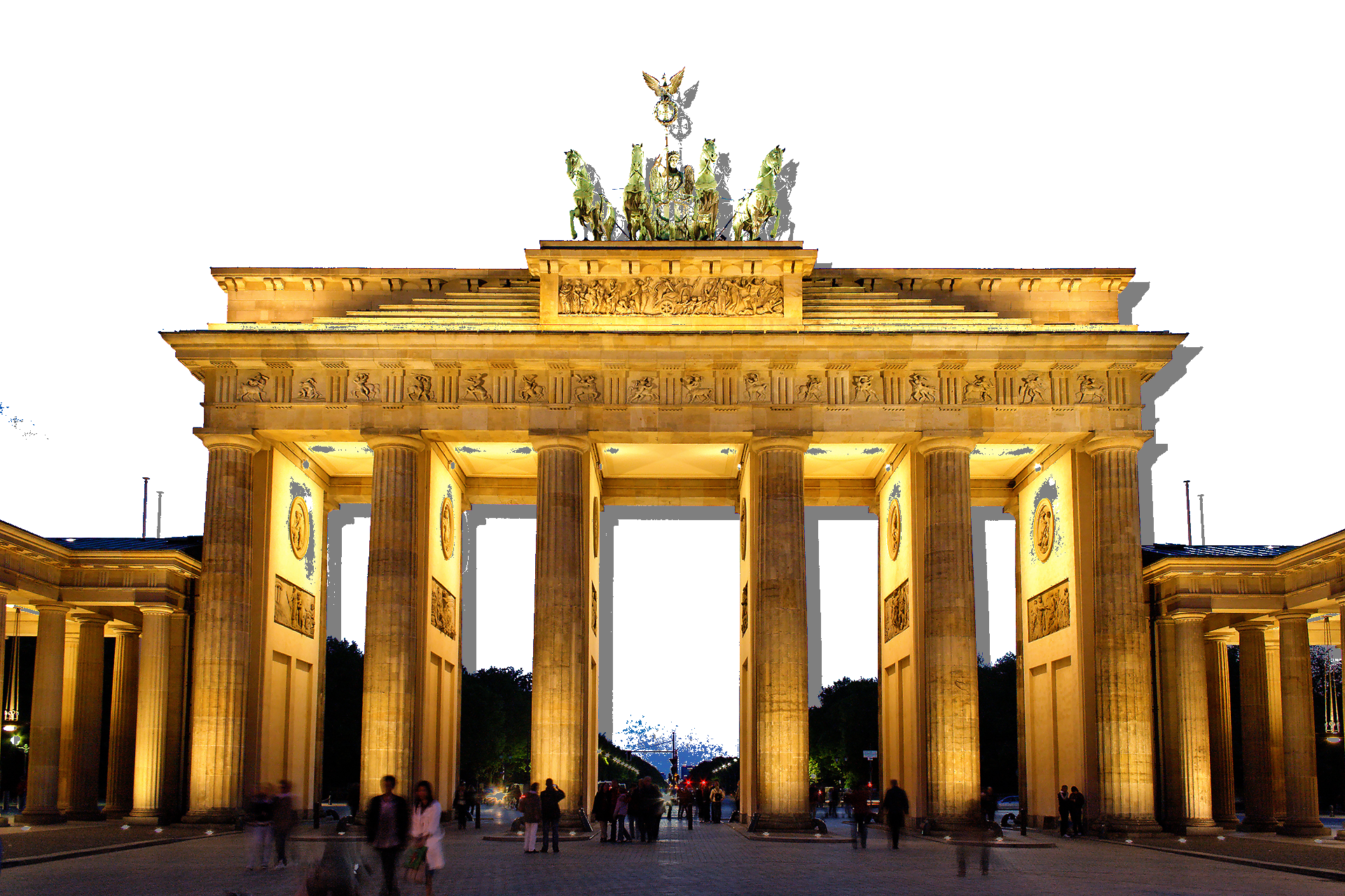

Core concepts

Concept 1 — Channel thresholds as content-aware masks

The mask in 3.2.1 was geometric — a circle around the centre. Here the mask is content-aware: it picks pixels by their colour. The blue channel of an RGB image is brightest where the sky lives (low red, low green, high blue), so a one-channel comparison gives a usable sky mask for free [2].

sky_mask = photo[:, :, 2] > 180     # shape (H, W), dtype bool

The choice of 180 is empirical — high enough to exclude the blue stones of the building, low enough to catch most of the sky gradient. As the README warns, some blue pixels do not turn white because changing the threshold would distort the gate too much. That is the standard trade-off for any single-channel threshold: tuning means picking the level that loses the least of what you care about.

Concept 2 — The silhouette layer

The trick that makes the shadow visible is a second image — same shape as the photo — that is uniform grey outside the mask and uniform white inside it. The mask is the same sky_mask we just built, so the silhouette layer is the negative of the subject:

shadow = np.full(photo.shape, 127, dtype=np.uint8)
shadow[sky_mask] = 255     # white where the sky is, grey everywhere else

The grey area is the subject’s silhouette; the white area is its complement. Translating the whole layer moves the silhouette boundary, and only the boundary will ever be visible in the final composite — the white-on-white overlap inside the sky is invisible, and the grey-on-photo overlap stays out of the masked region.

Concept 3 — Translating by slice assignment

A naive translation creates a new array (e.g. np.roll) or padding wraps the content across the edges. The slicing trick avoids both:

shadow[20:, 20:] = shadow[:-20, :-20]

The right-hand side is a view of the original layer minus its last 20 rows and columns; the left-hand side is the same shape, anchored 20 pixels down and 20 right. The result is an in-place translation: every pixel in the visible region moves down-and-right, and the top 20 rows and left 20 columns retain their original grey (which is exactly the boundary colour, so the seam is invisible) [3].

Concept 4 — Selective composite

The final step composites only inside the original mask. We never touch pixels that belong to the subject — only sky pixels can ever be repainted:

photo[sky_mask] = shadow[sky_mask]

shadow[sky_mask] indexes the translated silhouette at sky positions. Within the sky, most of those positions are white (which paints over the original sky as white), but the translated grey region — the shadow itself — sits over a small crescent of sky just behind the building, and those pixels become grey. The crescent is what you read as the cast shadow.

Exercises

Three exercises in Execute → Modify → Create order: run the script, tune three knobs, then build a coloured shadow.

shadow[60:, 60:] = shadow[:-60, :-60]

shadow = np.full(photo.shape, 64, dtype=np.uint8)
shadow[sky_mask] = 255

sky_mask = photo[:, :, 2] > 210

import numpy as np
from PIL import Image

photo = np.array(Image.open('bbtor.jpg'))
sky = photo[:, :, 2] > 180

# TODO 1: build a 3-channel shadow layer where the *base* colour is warm
#         (e.g. (220, 160, 120)) and the in-subject region is white.

# TODO 2: translate the whole layer by (30, 30) using slice assignment on all 3 channels.

# TODO 3: composite back into photo *inside the sky mask only*.

Image.fromarray(photo).save('warm_shadow.png')

shadow = np.full(photo.shape, [220, 160, 120], dtype=np.uint8)
shadow[sky] = [255, 255, 255]

shadow[30:, 30:] = shadow[:-30, :-30]

import numpy as np
from PIL import Image

photo = np.array(Image.open('bbtor.jpg'))
sky = photo[:, :, 2] > 180

# Warm grey-orange outside the subject; white inside
shadow = np.full(photo.shape, [220, 160, 120], dtype=np.uint8)
shadow[sky] = [255, 255, 255]

# Translate the silhouette by 30 px down-and-right
shadow[30:, 30:] = shadow[:-30, :-30]

# Composite back into the original photo, sky-only
photo[sky] = shadow[sky]

Image.fromarray(photo).save('warm_shadow.png')

Downloads

Summary

Common pitfalls to avoid

• np.roll instead of slicing — the bottom rows wrap onto the top and you get rogue building bits floating in the sky.
• Indexing the original sky mask after the composite — the sky has been overwritten, so photo[:, :, 2] > 180 no longer holds. Cache the mask once and reuse it.
• A mask that is (H, W, 3) instead of (H, W) — every operation in this lesson assumes 2D.
• Letting the silhouette layer share dtype=float with the photo’s uint8 — the assignment crashes or silently truncates. Use the same dtype in both arrays.
• Painting the silhouette layer everywhere instead of through the mask — you flood the building with grey too.

References

- [1] Porter, T., & Duff, T. (1984). Compositing digital images. ACM SIGGRAPH Computer Graphics, 18(3), 253–259. doi:10.1145/964965.808606
- [2] Gonzalez, R. C., & Woods, R. E. (2018). Digital Image Processing (4th ed.). Pearson.
- [3] Harris, C. R., Millman, K. J., van der Walt, S. J., et al. (2020). Array programming with NumPy. Nature, 585, 357–362. doi:10.1038/s41586-020-2649-2
- [4] NumPy Community. (2024). numpy.roll. NumPy Documentation. numpy.org
- [5] Bornstein, M. H. (1973). The psychophysiological component of cultural difference in colour naming and illusion susceptibility. Behavior Science Notes, 8, 41–101.
- [6] Reinhard, E., Khan, E. A., Akyüz, A. O., & Johnson, G. M. (2008). Color Imaging: Fundamentals and Applications. CRC Press.