3.4.2 Sobel Edge Detection
Specialise convolution into a gradient operator. Two 3×3 kernels — one measuring horizontal change, one measuring vertical — combine via Euclidean magnitude into an orientation-independent edge map.
Overview
The previous lesson’s “edge detection” kernel was a single 3×3 grid that fires wherever the centre pixel differs from its neighbours. The Sobel operator, developed by Irwin Sobel at Stanford in 1968 [1], does something more refined: it splits the question into horizontal and vertical gradient measurements with two separate kernels, then recombines them via the gradient magnitude √(Gₓ² + Gᵧ²). The result is an orientation-independent edge map that handles diagonal boundaries as cleanly as axis-aligned ones [2]. The same Sobel kernels live inside every modern edge detector, from the Canny algorithm to the convolutional stages of deep object-detection networks.
Learning objectives
- Read and apply the Sobel
GₓandGᵧkernels — one measures rate of change along x, the other along y. - Combine the two gradient images into a magnitude map with
√(Gₓ² + Gᵧ²). - Threshold the magnitude to isolate strong edges from background noise.
- Compare Sobel to Prewitt (equal-weight neighbours) and Roberts (2×2 cross) operators.
Quick start — Sobel on geometric shapes
import numpy as np
from PIL import Image

H, W = 256, 256
image = np.zeros((H, W), dtype=np.float64)
image[80:180, 60:120] = 255                          # rectangle

y, x = np.ogrid[:H, :W]
image[(x - 180) ** 2 + (y - 128) ** 2 <= 40 ** 2] = 255   # circle

# The two Sobel kernels
Gx = np.array([[-1, 0, 1],
               [-2, 0, 2],
               [-1, 0, 1]], dtype=np.float64)
Gy = np.array([[-1, -2, -1],
               [ 0,  0,  0],
               [ 1,  2,  1]], dtype=np.float64)

mag = np.zeros((H, W), dtype=np.float64)
for y_i in range(1, H - 1):
    for x_i in range(1, W - 1):
        n = image[y_i - 1:y_i + 2, x_i - 1:x_i + 2]
        gx = np.sum(Gx * n)
        gy = np.sum(Gy * n)
        mag[y_i, x_i] = np.hypot(gx, gy)             # √(gx² + gy²)

mag = (255 * mag / mag.max()).astype(np.uint8)
Image.fromarray(mag, 'L').save('edge_detection_output.png')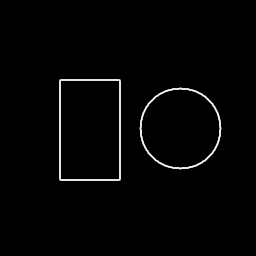
Core concepts
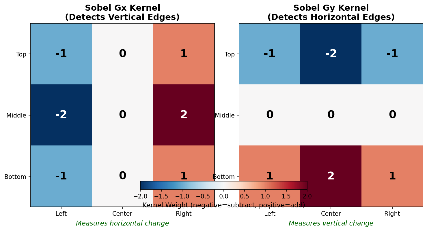
Concept 1 — The two Sobel kernels
The horizontal Sobel kernel Gₓ measures the rate of change along x — i.e. how much pixel value changes as you step rightward across the kernel:
        | -1   0   1 |
Gₓ  =   | -2   0   2 |
        | -1   0   1 |
Positive on the right, negative on the left, zero in the middle. In a uniform region the positives and negatives cancel. At a vertical edge — a sharp change from dark to bright as you move right — they reinforce. The “1-2-1” weighting along the centre row is the Sobel signature: it weighs the immediate row above and below more than the far neighbours, which doubles as a small Gaussian-like smoothing along the perpendicular axis [1].
The vertical Sobel kernel Gᵧ is the same kernel rotated 90°:
        | -1  -2  -1 |
Gᵧ  =   |  0   0   0 |
        |  1   2   1 |
Same logic, perpendicular direction.
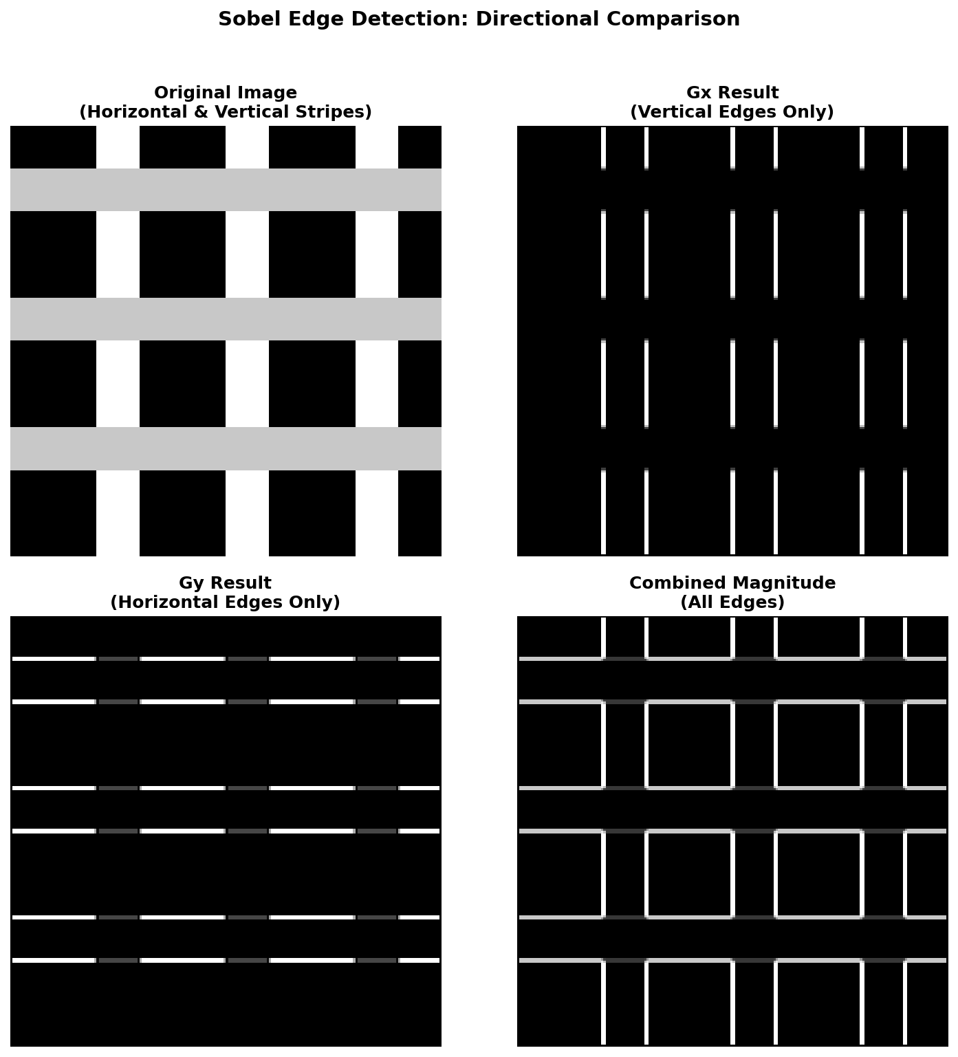
Concept 2 — Gradient magnitude
Convolving the image with each kernel gives two gradient images, Gₓ_image and Gᵧ_image. These are signed — a value is positive when intensity rises across the kernel, negative when it falls. To collapse direction into a single “edge strength” per pixel, take the Euclidean gradient magnitude |∇I| = sqrt(Gₓ² + Gᵧ²).
NumPy’s np.hypot(gx, gy) is the numerically-stable form of np.sqrt(gx*gx + gy*gy) — it avoids intermediate overflow when both gradients are large [3]. The result is non-negative and orientation-independent: a vertical, horizontal, or 45° edge all produce the same magnitude for the same intensity step.
Concept 3 — Sobel vs Prewitt vs Roberts
Three classical operators dominated edge detection in the 1960s-70s before Canny arrived. They differ only in the kernel weights [4, 5, 6]:
| Operator | Year | Kernel size | Gₓ weights |
|---|---|---|---|
| Roberts cross | 1965 | 2×2 | [[1, 0], [0, -1]] (diagonal pair only) |
| Prewitt | 1970 | 3×3 | [[-1, 0, 1], [-1, 0, 1], [-1, 0, 1]] (equal weights) |
| Sobel | 1968 | 3×3 | [[-1, 0, 1], [-2, 0, 2], [-1, 0, 1]] (centre row doubled) |
Roberts is fastest but noisy because it only samples two pixels. Prewitt and Sobel have similar quality; Sobel’s centre-weighted rows give it slightly smoother edges and a tiny Gaussian-like noise filter built in. The Canny detector (1986) layered Gaussian smoothing, Sobel-or-Prewitt gradient, non-maximum suppression, and hysteresis thresholding on top — it remains the gold standard [7].
Exercises
Three exercises in Execute → Modify → Create order: run the geometric shapes, restrict to one direction or threshold, then implement Sobel on a custom pattern.
Run the rectangle-and-circle test
Run simple_edge_detection.py from the downloads. The script generates the rectangle + circle test image, applies the Sobel pipeline, and saves the result.
Reflection questions
- Why do the insides of the rectangle and circle appear black?
- Are all four sides of the rectangle equally bright? Why or why not?
- Why does the circle, whose boundary is curved (no axis-aligned edges), still show up cleanly?
Answers
Interiors black — gradient measures change. Inside the rectangle and circle the pixels are all 255; the convolution sum is zero (the kernel’s positive and negative weights cancel). No change → no edge.
Four sides equally bright — the magnitude is orientation-independent. The left and right sides have high Gₓ and zero Gᵧ; the top and bottom have high Gᵧ and zero Gₓ. After √(Gₓ² + Gᵧ²) both directions produce the same magnitude. The corners go slightly higher because both gradients fire there.
Curved circle — at every point on the circle the local tangent has some angle θ. The local gradient is (Gₓ, Gᵧ) = (sinθ, cosθ) × step_size. The magnitude is step_size for every θ, so the whole circumference glows equally bright.
Three Sobel variations
Edit simple_edge_detection.py for each goal.
Goals
- Vertical edges only — use
|Gₓ|as the output, ignoreGᵧ. - Horizontal edges only — use
|Gᵧ|, ignoreGₓ. - Threshold — keep only edge pixels brighter than 30% of the maximum; set the rest to zero.
Goal 1 — what to expect
mag[y_i, x_i] = abs(gx)Only the left and right sides of the rectangle survive; the top and bottom vanish. The circle splits into two crescents — left and right curves visible, top and bottom invisible.
Goal 2 — what to expect
mag[y_i, x_i] = abs(gy)Mirror image: top/bottom rectangle, top/bottom circle.
Goal 3 — what to expect
threshold = 0.3 * mag.max()
mag[mag < threshold] = 0
Weak edges (anti-aliased curves, near-noise responses) drop out. The result looks like a binary edge map — sharp white lines on solid black, no grey gradient.
Sobel on a custom pattern
Build a procedural test image of your choice (a “T” shape, concentric rings, diagonal stripes — anything) and run the full Sobel pipeline on it. The output should clearly outline the pattern.
import numpy as np
from PIL import Image

H, W = 256, 256
image = np.zeros((H, W), dtype=np.float64)

# TODO 1: draw your pattern. Example: a "T" shape using rectangles.

# TODO 2: define Gx and Gy (you know what these are now).
# Gx = ...
# Gy = ...

# TODO 3: convolve and compute magnitude in nested loops.

# TODO 4: normalise to [0, 255] and save.

Image.fromarray(...).save('my_edges.png')
Hint 1 — pattern ideas
image[50:70, 80:180]   = 255    # horizontal bar of a "T"
image[60:180, 115:145] = 255    # vertical bar of a "T"
image[200:230, 200:230] = 200   # smaller dim accent square
Mix bright and dim regions so the edge magnitude varies across the picture — easier to see what Sobel is doing.
Hint 2 — the pipeline (same as quick start)
Gx = np.array([[-1, 0, 1], [-2, 0, 2], [-1, 0, 1]], dtype=np.float64)
Gy = np.array([[-1, -2, -1], [0, 0, 0], [1, 2, 1]], dtype=np.float64)

mag = np.zeros((H, W), dtype=np.float64)
for y in range(1, H - 1):
    for x in range(1, W - 1):
        n = image[y - 1:y + 2, x - 1:x + 2]
        mag[y, x] = np.hypot(np.sum(Gx * n), np.sum(Gy * n))
Complete solution
import numpy as np
from PIL import Image

H, W = 256, 256
image = np.zeros((H, W), dtype=np.float64)
image[50:70,  80:180]  = 255
image[60:180, 115:145] = 255
image[200:230, 200:230] = 200

Gx = np.array([[-1, 0, 1], [-2, 0, 2], [-1, 0, 1]], dtype=np.float64)
Gy = np.array([[-1, -2, -1], [0, 0, 0], [1, 2, 1]], dtype=np.float64)

mag = np.zeros((H, W), dtype=np.float64)
for y in range(1, H - 1):
    for x in range(1, W - 1):
        n = image[y - 1:y + 2, x - 1:x + 2]
        mag[y, x] = np.hypot(np.sum(Gx * n), np.sum(Gy * n))

mag = (255 * mag / mag.max()).astype(np.uint8)
Image.fromarray(mag, 'L').save('my_edges.png')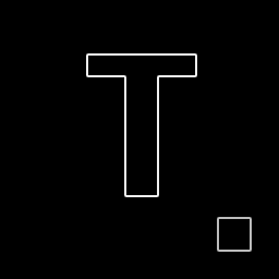
How it works:
- The pattern is just rectangle assignments on a
float64canvas. - The Sobel convolution is identical to Concept 1, applied with
np.hypotfor numerical stability. - The accent square’s edges are dimmer because its intensity step is
200rather than255— gradient magnitude scales with the size of the intensity change.
Make it your own
- Swap
Gx, Gyfor the Prewitt kernels ([[-1, 0, 1], [-1, 0, 1], [-1, 0, 1]]). Compare the outputs — they should be very similar. - Apply Sobel to each colour channel of an RGB image separately and combine the three magnitudes with
np.linalg.norm. The result is a colour-aware edge detector. - Pre-blur with the Gaussian kernel from 3.4.1 before running Sobel. This is the first stage of the Canny pipeline and produces much cleaner edges on noisy photos.
Downloads
simple_edge_detection.py — quick-start Sobel gradient_comparison.py — Gx/Gy comparison edge_detection_starter.py — Exercise 3 starter edge_detection_solution.py — Exercise 3 referenceSummary
Common pitfalls to avoid
- Calling
Gₓthe “horizontal-edge kernel” — it is the horizontal-gradient kernel, which detects vertical edges. - Using
np.sqrt(gx*gx + gy*gy)instead ofnp.hypot— both work for moderate inputs, buthypotis numerically stable for very large or very small magnitudes. - Forgetting to normalise — the raw magnitude often peaks above 1000, and
.astype(np.uint8)wraps modulo 256 instead of clipping. - Skipping the border — the 3×3 kernel cannot be centred on the outermost pixels. Either pad first (3.4.1) or loop from
(1, 1)to(H-1, W-1)and accept a 1-pixel ring of black. - Working in
uint8— the multiplication overflows immediately. Cast tofloat64before convolving.
References
- [1] Sobel, I., & Feldman, G. (1968). A 3×3 isotropic gradient operator for image processing. Talk at Stanford Artificial Intelligence Project (SAIL).
- [2] Gonzalez, R. C., & Woods, R. E. (2018). Digital Image Processing (4th ed.). Pearson.
- [3] NumPy Community. (2024). numpy.hypot. NumPy Documentation. numpy.org/hypot
- [4] Roberts, L. G. (1965). Machine perception of three-dimensional solids. In Optical and Electro-Optical Information Processing (pp. 159–197). MIT Press.
- [5] Prewitt, J. M. S. (1970). Object enhancement and extraction. In B. Lipkin & A. Rosenfeld (Eds.), Picture Processing and Psychopictorics (pp. 75–149). Academic Press.
- [6] Marr, D., & Hildreth, E. (1980). Theory of edge detection. Proceedings of the Royal Society of London. Series B, 207(1167), 187–217.
- [7] Canny, J. (1986). A computational approach to edge detection. IEEE Transactions on Pattern Analysis and Machine Intelligence, PAMI-8(6), 679–698. doi:10.1109/TPAMI.1986.4767851