3.4.1 Convolution

Overview

Convolution is the workhorse of image processing: slide a small matrix of weights (the kernel) across the image, compute the weighted sum of the pixels under the kernel at every position, and the output is a transformed image. The kernel’s values decide what the transformation does — equal weights give a blur, a positive centre with negative surround gives a sharpen, a sign-flipped surround gives edge detection [1]. The same operation runs the convolutional layer of a CNN, the Gaussian smoothing of every photo app, the unsharp mask of every printing pipeline. This lesson implements convolution from scratch with two nested loops, so the what-the-kernel-does intuition lives inside your hands.

Learning objectives

1. Implement 2D convolution from scratch: position the kernel, multiply element-wise, sum into the output pixel.
2. Read four canonical 3×3 kernels (identity, blur, sharpen, edge-detect) and predict their visual effect.
3. Pad the input with np.pad(..., mode='edge') to keep the output the same size as the input.
4. Clip vs normalise the output: pick the right post-processing for the kernel you used.

Quick start — blur a checkerboard

import numpy as np
from PIL import Image

SIZE = 256
TILE = 32

# Procedural checkerboard with sharp edges
rows = (np.arange(SIZE) // TILE)[:, None]
cols = (np.arange(SIZE) // TILE)[None, :]
canvas = np.where((rows + cols) % 2 == 0, 255.0, 0.0)

K = 5
blur = np.ones((K, K)) / (K * K)            # equal weights, sum to 1

# Convolution by nested loops (valid output: image - kernel + 1)
out_size = SIZE - K + 1
out = np.zeros((out_size, out_size))
for y in range(out_size):
    for x in range(out_size):
        region = canvas[y:y + K, x:x + K]
        out[y, x] = np.sum(region * blur)

Image.fromarray(out.astype(np.uint8), 'L').save('simple_convolution.png')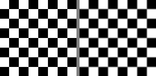

Core concepts

Concept 1 — Convolution in three steps

For a kernel K of size k × k and an input image I, the discrete 2D convolution at output position (y, x) sums the element-wise product over the k × k window:

O[y, x] = Σ_i Σ_j  I[y + i, x + j] · K[i, j]      for i, j in 0..k-1

Three steps per output pixel:

1. Position — pick the k × k region of the input centred on (or anchored at) the output pixel.
2. Multiply — element-wise multiply that region by the kernel.
3. Sum — add up the products. The total is the value of the output pixel [1].

Each output pixel is a single weighted average of its neighbourhood. The kernel’s weights are what the weighting is.

Concept 2 — Four canonical 3×3 kernels

Read the weights, predict the effect.

Identity — pass through.

identity = np.array([
    [0, 0, 0],
    [0, 1, 0],
    [0, 0, 0],
])

Only the centre pixel survives; every output equals its input. Useful as a sanity check.

Box blur — average.

blur = np.array([
    [1, 1, 1],
    [1, 1, 1],
    [1, 1, 1],
]) / 9.0

Equal weights, normalised to sum 1. Every output is the mean of the 3×3 neighbourhood. Sharp edges become 3-pixel ramps.

Sharpen — amplify the centre, subtract the neighbours.

sharpen = np.array([
    [ 0, -1,  0],
    [-1,  5, -1],
    [ 0, -1,  0],
])

Centre weighted 5; the four neighbours weighted -1. In a uniform region the negatives cancel 4 × (-1) × value + 5 × value = value — the picture passes through. At an edge, the negatives subtract less than they could, so the centre wins and the edge gets emphasised.

Edge detection — opposite sign on centre vs surround.

edge = np.array([
    [-1, -1, -1],
    [-1,  8, -1],
    [-1, -1, -1],
])

Sum is zero; constant regions go to zero. Only places where the centre differs from its neighbours produce non-zero output — the edges [2].

Concept 3 — Padding to keep output size

A naive convolution shrinks the output by kernel_size - 1 in each dimension — there’s no valid neighbourhood for output pixels near the edge. To keep the output the same size, pad the input with pad = kernel_size // 2 rows/columns of extra pixels before the loop:

pad = K // 2
padded = np.pad(image, pad, mode='edge')      # copy edge values outward
out = np.zeros_like(image, dtype=np.float64)
for y in range(image.shape[0]):
    for x in range(image.shape[1]):
        region = padded[y:y + K, x:x + K]
        out[y, x] = np.sum(region * kernel)

Three padding modes, all reasonable:

• mode='constant' (zero pad) — fills the border with zeros. Cheap; introduces dark fringe artefacts because the kernel “sees” black.
• mode='edge' — repeats the outermost row/column outward. The default in this module: preserves edge brightness, no artificial values.
• mode='reflect' — mirrors the image at the boundary. Smoothest visual continuation, slightly more expensive.

After convolution with a zero-sum kernel (sharpen, edge-detect), the output can go negative or exceed 255. Two recovery options:

clipped    = np.clip(out, 0, 255)                                   # fast
normalised = (out - out.min()) / (out.max() - out.min()) * 255      # full dynamic range

Use clipping when you only care about strong responses; normalise when you want every edge visible, including weak ones [1].

Exercises

Three exercises in Execute → Modify → Create order: run a 4-kernel comparison, swap kernels, then write your own convolve function with edge padding.

EXECUTE I.

Compare four kernels on the same photo

Run exercise1_execute.py from the downloads. It applies identity, blur, sharpen, and edge-detect to the Brandenburg Gate photograph and lays them out in a 2×2 grid.

Reflection questions

• Why does the identity kernel return the same image when its centre is 1 and everything else is 0?
• The edge-detection output is mostly black. Why?
• What would happen if you applied the blur kernel ten times in a row?

Answers

Identity — at every position, the convolution is 1 × centre_pixel + 0 × everything_else = centre_pixel. Each output equals its input.

Edges black — the edge-detection kernel sums to zero. In any constant region (the sky, the smooth parts of the columns), the sum is 8 × value + 8 × (-value) = 0. Only pixels at intensity transitions produce non-zero output, which is exactly where edges live.

Ten blurs — successive box blurs approximate a Gaussian blur, with the standard deviation growing as √n × σ_single. Ten 3×3 blurs is roughly equivalent to one Gaussian with σ ≈ √10 ≈ 3.2 pixels. The picture progressively dissolves into broad colour fields.

diag = np.array([
    [-1, -1,  0],
    [-1,  0,  1],
    [ 0,  1,  1],
])

stronger = np.array([
    [ 0, -2,  0],
    [-2,  9, -2],
    [ 0, -2,  0],
])

K = 5
blur = np.ones((K, K)) / (K * K)

CREATE III.

Same-size convolution with edge padding

Build a small convolve(image, kernel) function that pads the input with np.pad(..., mode='edge') so the output has exactly the same shape as the input. Apply it to the Brandenburg photo with a Gaussian-style kernel.

python · exercise3_starter.py Copy

import numpy as np
from PIL import Image

def convolve(image, kernel):
    """Same-size 2D convolution with edge-replicate padding."""
    H, W = image.shape
    K = kernel.shape[0]              # assume square kernel
    pad = K // 2

    # TODO 1: pad the image with mode='edge'.
    # TODO 2: allocate the output array.
    # TODO 3: nested loop over (y, x); accumulate the weighted sum.
    return output

# A 5×5 Gaussian-like kernel (Pascal's triangle outer product)
g = np.array([1, 4, 6, 4, 1])
gauss = np.outer(g, g) / np.sum(np.outer(g, g))

photo = np.array(Image.open('bbtor.jpg').convert('L'), dtype=np.float64)
blurred = convolve(photo, gauss)

Image.fromarray(np.clip(blurred, 0, 255).astype(np.uint8), 'L').save('gauss_blur.png')

Hint 1 — padding

padded = np.pad(image, pad, mode='edge')

The output of np.pad has shape (H + 2*pad, W + 2*pad). Indexing padded[y:y+K, x:x+K] will always be valid for y in range(H) and x in range(W).

Hint 2 — output shape and loop

output = np.zeros((H, W), dtype=np.float64)
for y in range(H):
    for x in range(W):
        output[y, x] = np.sum(padded[y:y + K, x:x + K] * kernel)

Note the loop is over the unpadded size; the padding is implicit in the index window.

Complete solution

python · exercise3_solution.py Copy

import numpy as np
from PIL import Image

def convolve(image, kernel):
    H, W = image.shape
    K = kernel.shape[0]
    pad = K // 2
    padded = np.pad(image, pad, mode='edge')

    output = np.zeros((H, W), dtype=np.float64)
    for y in range(H):
        for x in range(W):
            output[y, x] = np.sum(padded[y:y + K, x:x + K] * kernel)
    return output

# Pascal-triangle Gaussian-style 5×5
g = np.array([1, 4, 6, 4, 1])
gauss = np.outer(g, g)
gauss = gauss / gauss.sum()

photo = np.array(Image.open('bbtor.jpg').convert('L'), dtype=np.float64)
blurred = convolve(photo, gauss)

Image.fromarray(np.clip(blurred, 0, 255).astype(np.uint8), 'L').save('gauss_blur.png')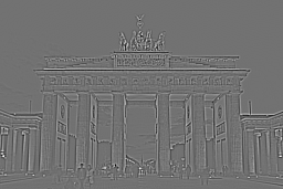

How it works:

• np.pad(image, pad, mode='edge') adds a pad-wide ring around the input by copying the border row/column outward.
• The loop indexes the padded image with offsets y..y+K (always valid by construction).
• Output shape matches the input because we loop over the original H × W range.
• The Gaussian-like kernel is the outer product of two Pascal’s-triangle rows; it sums to 1 after normalisation, so brightness is preserved.

Make it your own

• Replace np.sum(padded[y:y+K, x:x+K] * kernel) with (padded[y:y+K, x:x+K] * kernel).sum() and watch the timing — they are nearly identical, but scipy.signal.convolve2d is 50–100× faster than either Python loop.
• Apply the same convolve function to each colour channel of an RGB image and stack the three outputs.
• Combine a sharpen and a blur: convolve with the sharpen first, then convolve again with the blur. The result is unsharp masking — the standard technique for softening over-sharpened images.

Downloads

Summary

Common pitfalls to avoid

• Working in uint8 instead of float64 — multiplications overflow at 256 and the output is garbage. Cast to float64 first.
• Forgetting to normalise a blur kernel — without / K², the output overshoots by a factor of K² and saturates to white.
• Indexing the padded image with the original coordinates — off by pad. Loop over range(H) and index padded[y:y+K].
• Mixing up np.sum(a * b) and np.dot(a.ravel(), b.ravel()) — equivalent for matching shapes, but the dot product surprises beginners with shape errors.
• Reusing kernels across uint8 and float64 images — make sure the dtype is consistent end-to-end.

References

- [1] Gonzalez, R. C., & Woods, R. E. (2018). Digital Image Processing (4th ed.). Pearson.
- [2] Marr, D., & Hildreth, E. (1980). Theory of edge detection. Proceedings of the Royal Society of London. Series B, 207(1167), 187–217. doi:10.1098/rspb.1980.0020
- [3] LeCun, Y., Bottou, L., Bengio, Y., & Haffner, P. (1998). Gradient-based learning applied to document recognition. Proceedings of the IEEE, 86(11), 2278–2324. doi:10.1109/5.726791
- [4] Szeliski, R. (2022). Computer Vision: Algorithms and Applications (2nd ed.). Springer.
- [5] NumPy Community. (2024). numpy.pad. NumPy Documentation. numpy.org/pad
- [6] SciPy Community. (2024). scipy.signal.convolve2d. SciPy Documentation. docs.scipy.org