3.4.3 Contour Lines

Overview

A contour map turns a continuous 2D scalar field into a readable picture. Topographic maps use it for elevation; weather maps use it for pressure; medical images use it for tissue density. The same construction shows up everywhere a scientist wants to see level sets — the lines or bands along which a function takes a fixed value. Modern usage traces back to 18th-century French hydrographers mapping seabed depth; the principle stayed unchanged, and CT scans, marching cubes, and ggplot’s geom_contour all sit on top of it [1, 2]. This short lesson builds the field as a sum of Gaussian hills and renders it in the two canonical styles: stepped bands by integer quantisation, and thin isolines by a modulo test.

Learning objectives

1. Construct a 2D scalar field by summing a few Gaussian hills evaluated on a meshgrid.
2. Quantise the normalised field into N discrete levels with (normalised * N).astype(int) * (255 // N) for stepped contours.
3. Mark thin isolines using ((field * scale).round() % step) == 0 — one pixel wide.
4. Read the trade-off between number-of-levels and visual readability.

Quick start — one Gaussian hill

import numpy as np
from PIL import Image

SIZE = 300

x = np.linspace(-5, 5, SIZE)
y = np.linspace(-5, 5, SIZE)
X, Y = np.meshgrid(x, y)

# A single Gaussian hill centred at origin
height = np.exp(-(X**2 + Y**2) / 4)

# Normalise to [0, 1], quantise into 8 levels, rescale to [0, 255]
normalised = (height - height.min()) / (height.max() - height.min())
contour = (normalised * 8).astype(np.uint8) * 32     # 8 × 32 = 256 → wraps to 0
contour = np.clip(contour, 0, 255).astype(np.uint8)

Image.fromarray(contour, 'L').save('simple_contour.png')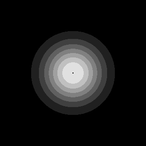

Core concepts

Concept 1 — Scalar fields and meshgrid

A scalar field is a function f(x, y) returning one value per (x, y) location. On a discrete grid it is exactly a 2D NumPy array. np.meshgrid is the standard tool for building the coordinate inputs:

x = np.linspace(-5, 5, 300)
y = np.linspace(-5, 5, 300)
X, Y = np.meshgrid(x, y)        # both shape (300, 300)

X[i, j] is the x-coordinate at pixel (i, j); Y[i, j] is its y-coordinate. With those two arrays, any scalar function can be evaluated for every pixel at once:

height = np.exp(-(X**2 + Y**2) / 4)         # Gaussian hill
distance = np.sqrt(X**2 + Y**2)             # distance field (same as 2.2.4)
spiral = np.sin(np.arctan2(Y, X) * 5 + distance)

Building maps of Z = f(X, Y) is the basic move; the contour styles in the next two concepts are different ways to visualise the same Z [3].

Concept 2 — Stepped bands by quantisation

Integer division turns a continuous range into discrete buckets. Apply the same idea to a normalised field:

normalised = (height - height.min()) / (height.max() - height.min())   # [0, 1]
levels = (normalised * N).astype(np.uint8)                              # 0..N-1
contour = levels * (255 // N)                                            # back to display range

Each pixel lands in exactly one of N buckets; pixels in the same bucket share the same grey value. The boundaries between buckets — the contours — are visible as the sharp lines between two grey levels. N = 8 gives a friendly stepped map; N = 4 gives bold poster-style bands; N = 64 looks almost continuous.

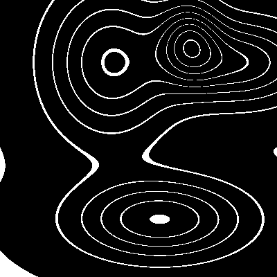
Concept 3 — Thin isolines via modulo

Stepped bands are everywhere except exactly on the boundaries. The traditional topographic-map style is the opposite — thin curves on the level set, blank everywhere else. The trick is a modulo test:

isolines = ((normalised * 100).round() % 16) == 0
isolines = (isolines * 255).astype(np.uint8)

Multiply the field by 100, round to the nearest integer, and check which values are exact multiples of step = 16. Those pixels become white; everything else stays black. The lines are 1-pixel wide because the rounded integer only equals a multiple at the discrete locations where the field crosses each threshold.

Tighter spacing comes from a smaller step (more lines); a higher scale means more granularity. The two work together — (scale, step) = (100, 16) gives ~6 levels across [0, 1]; (200, 20) gives ~10 levels [4].

Exercises

Three exercises in Execute → Modify → Create order: render both styles, vary the level count, then sum random hills into a richer terrain.

EXECUTE I.

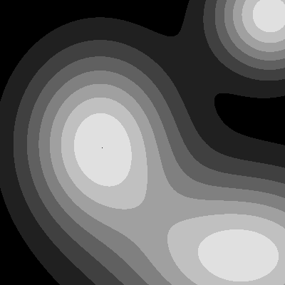
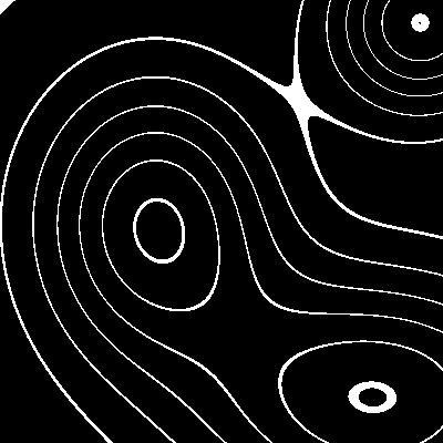
Render both styles

Run contour.py from the downloads. It builds a three-hill terrain (sum of three Gaussians) and saves both stepped contours and isolines as separate PNGs.

Reflection questions

• The hills overlap; in the stepped contour their joint region shows broad bands. Why are the bands wider there than in the isolated parts of each hill?
• The isolines are closed curves. Will they ever cross each other? Why or why not?
• What is the visual signature of a steep hill vs a gentle hill in the isoline picture?

Answers

Wider bands at overlap — where two hills overlap, the sum of two Gaussians is locally close to flat (both functions near their respective peaks contribute high values, and the gradient of the sum is small). Wider bands mean a smaller gradient — the field changes slowly across more pixels.

Isolines never cross — two isolines correspond to two different level values. For them to cross, the same pixel would have to take both values simultaneously, which is impossible for a single-valued field. They can be tangent (touch and bounce) but never transverse.

Steep vs gentle — steep hills produce tightly spaced isolines (the field crosses many levels in a small distance); gentle hills produce widely spaced isolines. The same convention used by hikers reading a topographic map.

contour = (znorm * 16).astype(np.uint8) * 16     # 16 × 16 = 256

contour = (znorm * 4).astype(np.uint8) * 64

isolines = ((znorm * 100).round() % 8) == 0

CREATE III.

A random terrain of hills

Build a terrain by summing 15 random Gaussian hills with varied positions, amplitudes, and widths. Render both styles.

python · exercise3_starter.py Copy

import numpy as np
from PIL import Image

SIZE = 400
N_HILLS = 15
rng = np.random.default_rng(0)

x = np.linspace(-10, 10, SIZE)
y = np.linspace(-10, 10, SIZE)
X, Y = np.meshgrid(x, y)

Z = np.zeros_like(X)

# TODO 1: for each of N_HILLS, sample random (cx, cy, amplitude, width)
#         and add an exp(-((X-cx)**2 + (Y-cy)**2) / width) term to Z.

# TODO 2: normalise Z to [0, 1].

# TODO 3: save the stepped contour (8 levels) AND the isolines.

Image.fromarray(stepped, 'L').save('random_terrain.png')
Image.fromarray(isolines, 'L').save('random_terrain_isolines.png')

Hint 1 — sum random hills

for _ in range(N_HILLS):
    cx = rng.uniform(-9, 9)
    cy = rng.uniform(-9, 9)
    amp = rng.uniform(0.5, 2.0)
    width = rng.uniform(1.5, 4.0)
    Z = Z + amp * np.exp(-((X - cx) ** 2 + (Y - cy) ** 2) / width)

Each iteration adds one Gaussian to the field. Different amp values make some peaks tall and some low; different width values make some narrow and some sprawling.

Hint 2 — render both styles

znorm = (Z - Z.min()) / (Z.max() - Z.min())
stepped = ((znorm * 8).astype(np.uint8) * 32).clip(0, 255).astype(np.uint8)
isolines = (((znorm * 100).round() % 12) == 0).astype(np.uint8) * 255

Both rendered styles take the same znorm; only the visualisation step differs.

Complete solution

python · exercise3_solution.py Copy

import numpy as np
from PIL import Image

SIZE = 400
N_HILLS = 15
rng = np.random.default_rng(0)

x = np.linspace(-10, 10, SIZE)
y = np.linspace(-10, 10, SIZE)
X, Y = np.meshgrid(x, y)

Z = np.zeros_like(X)
for _ in range(N_HILLS):
    cx, cy = rng.uniform(-9, 9, size=2)
    amp = rng.uniform(0.5, 2.0)
    width = rng.uniform(1.5, 4.0)
    Z = Z + amp * np.exp(-((X - cx) ** 2 + (Y - cy) ** 2) / width)

znorm = (Z - Z.min()) / (Z.max() - Z.min())

stepped = ((znorm * 8).astype(np.uint8) * 32).clip(0, 255).astype(np.uint8)
isolines = (((znorm * 100).round() % 12) == 0).astype(np.uint8) * 255

Image.fromarray(stepped, 'L').save('random_terrain.png')
Image.fromarray(isolines, 'L').save('random_terrain_isolines.png')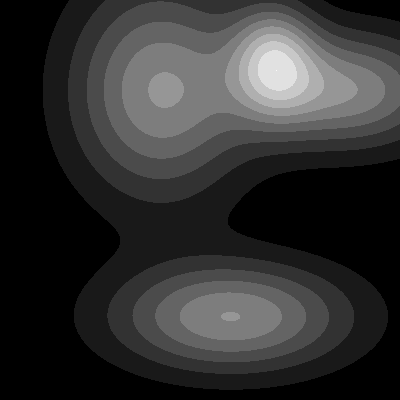

How it works:

• Each random hill is one Gaussian exp(-((X-cx)² + (Y-cy)²) / width); the field is their sum.
• Normalising to [0, 1] makes the quantisation step independent of the random amplitudes — even with totally different hills you get 8 levels.
• The two render styles are pure NumPy expressions, each one line.

Make it your own

• Replace the Gaussian hills with exp(-d) where d is computed with the Manhattan or Chebyshev metric. The level sets stop being circles and start being squares or diamonds.
• Render the stepped contour in colour by indexing a matplotlib colormap with the level array: cm.terrain(levels / 8).
• Animate the field over time — make the hill amplitudes a function of sin(2π·t/T) and save a GIF. The contours pulse like a slow-motion lava lamp.

Downloads

Summary

Common pitfalls to avoid

• Forgetting to normalise — without (z - z.min()) / (z.max() - z.min()), the quantisation depends on the absolute range of z and can produce a uniform black image.
• Casting before scaling — (field * 8).astype(int) * 256 overflows because 8 × 256 = 2048. Scale by (255 // N), not 256.
• Using int(x % 16 == 0) on a single float — works for one pixel, but for a NumPy array use (field % 16 == 0) to get the boolean array.
• Isolines too dense — % 2 == 0 against (field * 100) gives 50 levels and the picture turns into solid white.
• Mixing np.meshgrid indexing conventions — by default meshgrid returns X, Y with Y first along axis 0. If your hills appear rotated, swap (X, Y) to (Y, X).

References

- [1] USGS. (2024). Topographic Maps. USGS Education. usgs.gov
- [2] Lorensen, W. E., & Cline, H. E. (1987). Marching cubes: A high-resolution 3D surface construction algorithm. ACM SIGGRAPH Computer Graphics, 21(4), 163–169. doi:10.1145/37402.37422
- [3] Harris, C. R., Millman, K. J., van der Walt, S. J., et al. (2020). Array programming with NumPy. Nature, 585, 357–362. doi:10.1038/s41586-020-2649-2
- [4] Hunter, J. D. (2007). Matplotlib: A 2D graphics environment. Computing in Science & Engineering, 9(3), 90–95.
- [5] Slocum, T. A., McMaster, R. B., Kessler, F. C., & Howard, H. H. (2009). Thematic Cartography and Geovisualization (3rd ed.). Pearson.
- [6] Gonzalez, R. C., & Woods, R. E. (2018). Digital Image Processing (4th ed.). Pearson.