3.3.5 Delaunay Triangulation

Overview

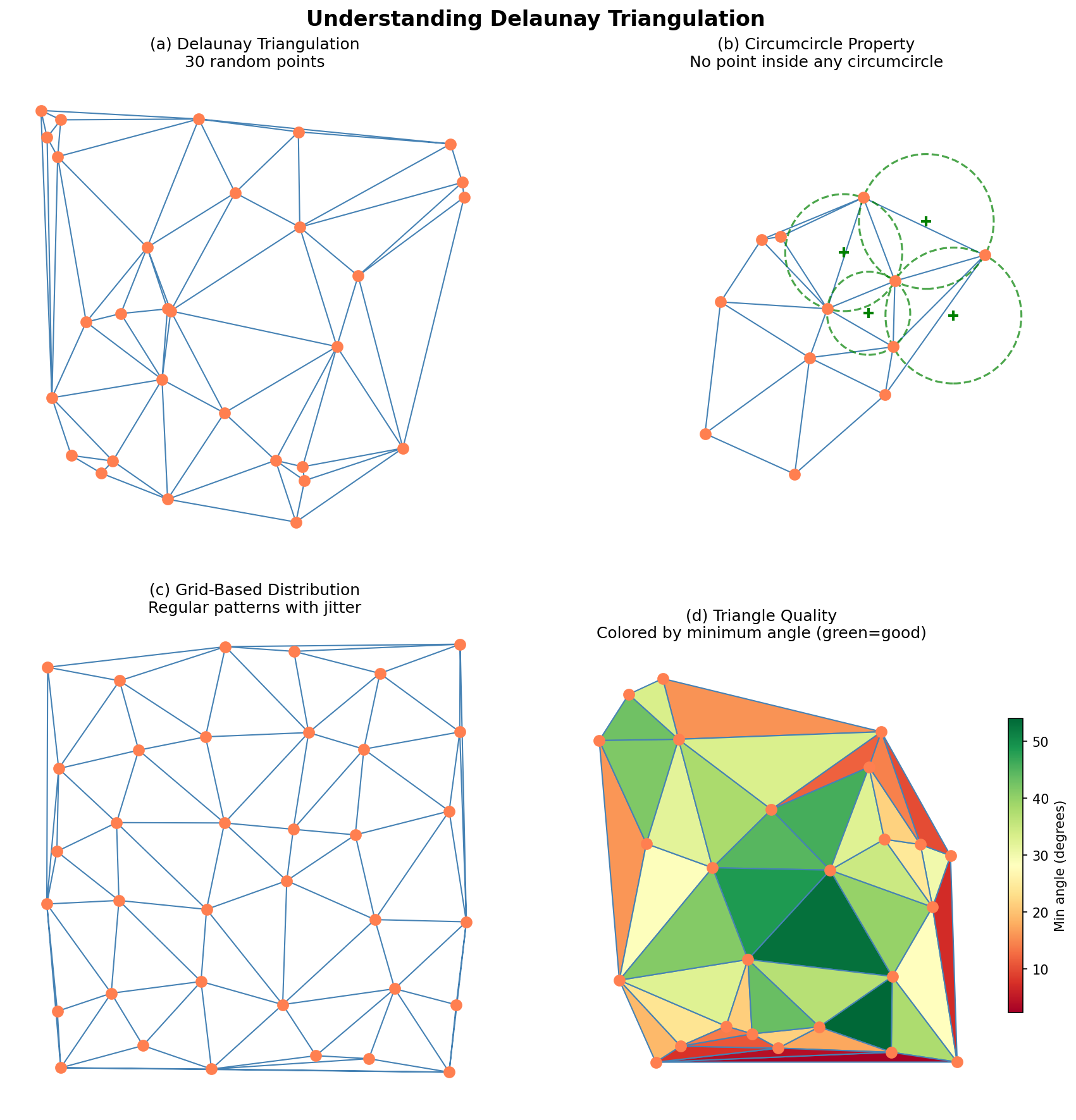
A Delaunay triangulation connects a point cloud into triangles such that no point sits inside any other triangle’s circumcircle. The constraint is elegant: out of the many ways to triangulate the same point set, this one maximises the smallest angle across all triangles — slivers are avoided and the mesh feels visually balanced [1]. Borrowed by graphics from finite-element meshing, Delaunay is now the standard triangulation for terrain generation, low-poly art, and the “facets” filter in every photo app. Boris Delaunay published the theorem in 1934; scipy.spatial.Delaunay packages it into one constructor call [2, 3].

Learning objectives

1. State the circumcircle property and explain why it produces well-shaped triangles.
2. Compute a triangulation with scipy.spatial.Delaunay(points) and read out its .simplices index array.
3. Sample colours from an image at each triangle’s centroid to render a low-poly facet image.
4. Compare point-distribution strategies — random, jittered grid, edge-weighted — for different artistic effects.

Quick start — triangulate 50 points

import numpy as np
import matplotlib.pyplot as plt
from scipy.spatial import Delaunay

rng = np.random.default_rng(42)
points = rng.random((50, 2)) * 400

tri = Delaunay(points)

fig, ax = plt.subplots(figsize=(7, 7))
ax.triplot(points[:, 0], points[:, 1], tri.simplices,
           color='steelblue', linewidth=0.8)
ax.plot(points[:, 0], points[:, 1], 'o', color='coral', markersize=6)
ax.set_aspect('equal'); ax.axis('off')
plt.savefig('simple_delaunay.png', dpi=150, bbox_inches='tight')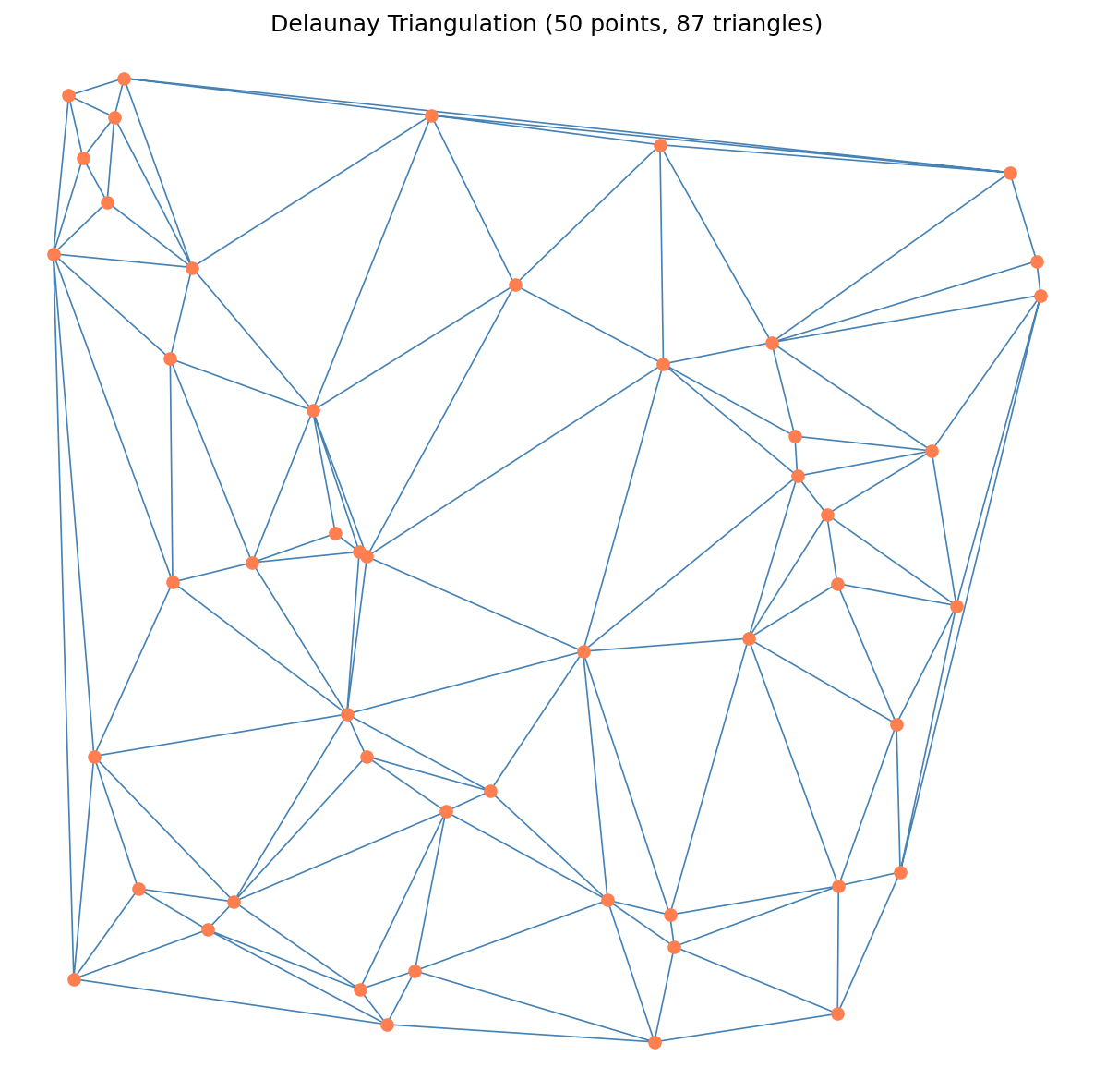

Core concepts

Concept 1 — The circumcircle property

Given a point cloud P, the Delaunay triangulation of P is the unique triangulation in which no point of P sits inside any triangle’s circumcircle (the unique circle passing through the triangle’s three vertices) [4]. Equivalently — and this is the property practitioners actually care about — Delaunay maximises the minimum angle over all triangles. There are no long thin slivers; every triangle is reasonably “fat.”

Why does that matter? Three reasons:

• Numerical stability — finite-element solvers, interpolation, gradient estimation all blow up on slivers.
• Visual balance — a mesh full of fat triangles looks intentional; one full of slivers looks broken.
• Mesh quality — Delaunay is the closest you get to “good triangles” without picking points yourself.

Concept 2 — Indexing into tri.simplices

tri.simplices is the canonical Delaunay output: a (num_triangles, 3) array of integer indices into your original point array. The first triangle has vertices points[tri.simplices[0]], the second has points[tri.simplices[1]], and so on. Two common operations:

# Pull out the three vertex coordinates for triangle k
triangle_k = points[tri.simplices[k]]      # shape (3, 2)

# Iterate over all triangles
for simplex in tri.simplices:
    vertices = points[simplex]              # (3, 2)
    centroid = vertices.mean(axis=0)        # (2,)
    ...

This index-then-look-up pattern is exactly the same one used by Warhol’s palette indexing in 3.3.1 — store integer references, fetch the data separately. It is also how OBJ, glTF, and every other indexed-mesh file format works.

Concept 3 — Centroid sampling for low-poly art

Once you have triangles, painting them by colour-sampling a source image is the “low-poly art” technique:

def triangle_colour(source, vertices):
    centroid = vertices.mean(axis=0)
    cx = int(np.clip(centroid[0], 0, source.shape[1] - 1))
    cy = int(np.clip(centroid[1], 0, source.shape[0] - 1))
    return source[cy, cx] / 255.0           # NB: image indexing is [y, x]

Centroid sampling is the cheapest variant — one pixel lookup per triangle. Better-looking versions average all pixels inside the triangle (use matplotlib.path.Path to test inclusion), but the centroid is enough for the geometric mosaic look [5].

The image gets rendered through matplotlib.collections.PolyCollection, which paints filled polygons in one call:

from matplotlib.collections import PolyCollection
triangles = [points[s] for s in tri.simplices]
colours   = [triangle_colour(source, points[s]) for s in tri.simplices]
ax.add_collection(PolyCollection(triangles, facecolors=colours, edgecolors='none'))
ax.set_xlim(0, W); ax.set_ylim(H, 0)        # flip y so image-down stays down

Exercises

Three exercises in Execute → Modify → Create order: run the wireframe, try different distributions, then render a low-poly image from a procedural source.

gx, gy = np.meshgrid(np.linspace(0, 400, 7), np.linspace(0, 400, 7))
points = np.column_stack([gx.ravel(), gy.ravel()])
points += rng.normal(0, 5, size=points.shape)

points = rng.beta(0.5, 0.5, size=(50, 2)) * 400

points = np.vstack([points, [[0, 0], [400, 0], [400, 400], [0, 400]]])

CREATE III.

Low-poly art from a procedural source

Build a procedural sunset image (gradient + sun + accent circle), generate a triangulation with corner+edge anchors, and render the low-poly version.

python · exercise3_starter.py Copy

import numpy as np
import matplotlib.pyplot as plt
from matplotlib.collections import PolyCollection
from scipy.spatial import Delaunay

W, H = 400, 400
rng = np.random.default_rng(42)

# TODO 1: build a procedural source image (H, W, 3) uint8 with a sunset gradient
#         and a sun-like circle. See hint for one approach.

# TODO 2: sample 150 random points, then append the 4 corners and 4 edge midpoints.

# TODO 3: compute the Delaunay triangulation.

# TODO 4: per triangle: sample the centroid colour from the source.

# TODO 5: render with PolyCollection; flip the y-axis to match image coords.

plt.savefig('lowpoly.png', dpi=150, bbox_inches='tight', pad_inches=0)

Hint 1 — procedural sunset

y, x = np.ogrid[:H, :W]
source = np.zeros((H, W, 3), dtype=np.uint8)
source[..., 0] = np.clip(255 - y * 0.4, 0, 255)
source[..., 1] = np.clip(100 + np.sin(x * 0.02) * 80, 0, 255)
source[..., 2] = np.clip(50 + y * 0.5, 0, 255)

# Add a sun in the upper portion
dist = np.sqrt((x - W // 2) ** 2 + (y - H // 3) ** 2)
sun = dist < 80
source[sun] = [255, 200, 80]

Hint 2 — points + anchors

points = rng.random((150, 2)) * [W, H]
corners = np.array([[0, 0], [W, 0], [W, H], [0, H]])
edges   = np.array([[W/2, 0], [W/2, H], [0, H/2], [W, H/2]])
points  = np.vstack([points, corners, edges])

The 8 extra points guarantee the hull covers the full canvas.

Hint 3 — render with PolyCollection

tri = Delaunay(points)

def tri_colour(simplex):
    verts = points[simplex]
    cx, cy = verts.mean(axis=0)
    cx = int(np.clip(cx, 0, W - 1)); cy = int(np.clip(cy, 0, H - 1))
    return source[cy, cx] / 255.0

triangles = [points[s] for s in tri.simplices]
colours   = [tri_colour(s)   for s in tri.simplices]

fig, ax = plt.subplots(figsize=(8, 8))
ax.add_collection(PolyCollection(triangles, facecolors=colours, edgecolors='none'))
ax.set_xlim(0, W); ax.set_ylim(H, 0); ax.set_aspect('equal'); ax.axis('off')

Complete solution

python · exercise3_solution.py Copy

import numpy as np
import matplotlib.pyplot as plt
from matplotlib.collections import PolyCollection
from scipy.spatial import Delaunay

W, H = 400, 400
rng = np.random.default_rng(42)

y, x = np.ogrid[:H, :W]
source = np.zeros((H, W, 3), dtype=np.uint8)
source[..., 0] = np.clip(255 - y * 0.4, 0, 255)
source[..., 1] = np.clip(100 + np.sin(x * 0.02) * 80, 0, 255)
source[..., 2] = np.clip(50 + y * 0.5, 0, 255)

dist = np.sqrt((x - W // 2) ** 2 + (y - H // 3) ** 2)
source[dist < 80] = [255, 200, 80]

points = rng.random((150, 2)) * [W, H]
corners = np.array([[0, 0], [W, 0], [W, H], [0, H]])
edges   = np.array([[W/2, 0], [W/2, H], [0, H/2], [W, H/2]])
points  = np.vstack([points, corners, edges])

tri = Delaunay(points)

def tri_colour(simplex):
    verts = points[simplex]
    cx, cy = verts.mean(axis=0)
    cx = int(np.clip(cx, 0, W - 1)); cy = int(np.clip(cy, 0, H - 1))
    return source[cy, cx] / 255.0

triangles = [points[s]   for s in tri.simplices]
colours   = [tri_colour(s) for s in tri.simplices]

fig, ax = plt.subplots(figsize=(8, 8))
ax.add_collection(PolyCollection(triangles, facecolors=colours, edgecolors='none'))
ax.set_xlim(0, W); ax.set_ylim(H, 0); ax.set_aspect('equal'); ax.axis('off')
plt.savefig('lowpoly.png', dpi=150, bbox_inches='tight', pad_inches=0)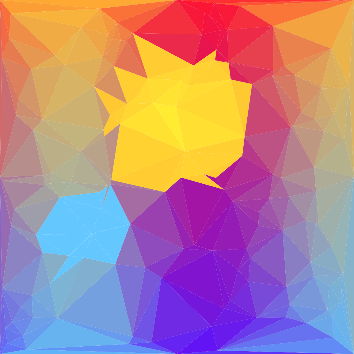

How it works:

• The source image is a normal NumPy array; nothing about Delaunay sees the pixels directly.
• Per-triangle centroid sampling picks one colour per triangle. The colour is a function of only the centroid, so adjacent triangles can be very different colours even if the underlying gradient is smooth.
• PolyCollection is matplotlib’s batch polygon renderer — one call paints all triangles at their respective colours.

Make it your own

• Replace centroid sampling with average sampling — use matplotlib.path.Path(triangle).contains_points to find the pixels inside each triangle and take their mean colour. Slower but visually closer to the source.
• Bias point placement by image gradient — sample more points where the source has sharp edges, fewer where it is smooth. Photo apps do this for “smart” low-poly conversion.
• Render the wireframe on top of the colour fill (edgecolors='white') for a stained-glass look. Drop the alpha (alpha=0.6) to layer it on top of the original image.

Downloads

Summary

Common pitfalls to avoid

• Forgetting corner anchors — the convex hull leaves border regions uncovered.
• Indexing the source as source[cx, cy] instead of source[cy, cx] — NumPy images are [row, col].
• Passing the vertices (points[s]) to a function expecting indices (s) or vice versa.
• Plotting without ax.set_ylim(H, 0) — the picture renders upside-down because matplotlib defaults to y-up.
• Sampling colours as source[cy, cx] without np.clip — points can land just outside the image bounds and crash the indexing.

References

- [1] Aurenhammer, F., Klein, R., & Lee, D.-T. (2013). Voronoi Diagrams and Delaunay Triangulations. World Scientific.
- [2] Delaunay, B. (1934). Sur la sphère vide. Bulletin de l’Académie des Sciences de l’URSS, Classe des Sciences Mathématiques et Naturelles, 6, 793–800.
- [3] SciPy Community. (2024). scipy.spatial.Delaunay. SciPy Documentation. docs.scipy.org
- [4] de Berg, M., Cheong, O., van Kreveld, M., & Overmars, M. (2008). Computational Geometry: Algorithms and Applications (3rd ed.). Springer.
- [5] Edelsbrunner, H. (2001). Geometry and Topology for Mesh Generation. Cambridge University Press.
- [6] Hunter, J. D. (2007). Matplotlib: A 2D graphics environment. Computing in Science & Engineering, 9(3), 90–95. doi:10.1109/MCSE.2007.55