3.3.3 Hexpanda — Hexbin Image Filter

Overview

Hexagonal binning is a tool from statistical graphics: every data point gets dropped into the nearest hexagonal cell, and each cell is coloured by how many points it caught. Originally Dan Carr designed it in 1987 to render scatter plots of millions of points without saturating the canvas [1]. The clever filter trick is to flip that pipeline backwards — treat every dark pixel of a photograph as a data point, sample a fraction of them, and plot the result with pandas.DataFrame.plot.hexbin. The picture comes back as a hex-mosaic version of the original, with detail abstracted into density and edges turned into honeycomb seams [2]. This is a short lesson that bridges NumPy image work to the pandas/matplotlib ecosystem you will use throughout Modules 7 and 14.

Learning objectives

1. Convert a grayscale image into an (x, y, intensity) DataFrame using unstack + reset_index.
2. Invert pixel values so dark image regions map to high-density hexagons.
3. Tune gridsize to trade detail for abstraction in the hexbin output.
4. Swap the matplotlib colormap (Greys, viridis, plasma, Blues) to change the visual mood.

Quick start — the hexpanda

import pandas as pd
import matplotlib.pyplot as plt
import numpy as np
from PIL import Image

# Grayscale + invert so dark → high value
pixels = np.array(Image.open('panda.png').convert('L'))
inverted = 255 - pixels

# Pixel grid → long-format DataFrame (x, y, intensity)
df = pd.DataFrame(inverted).unstack()             # (x, y) → intensity Series
df = df[df > 0].reset_index()                     # drop background, become flat
df.columns = ['x', 'y', 'intensity']
df['y'] = -df['y']                                # flip to maths y-up

# Sample 25% for an airier mosaic, then hexbin
sample = df.sample(len(df) // 4, random_state=0)

fig, ax = plt.subplots(figsize=(8, 8))
sample.plot.hexbin(x='x', y='y', gridsize=30, cmap='Greys', ax=ax)
ax.set_aspect('equal'); ax.axis('off')
plt.savefig('hexpanda.png', bbox_inches='tight', dpi=120)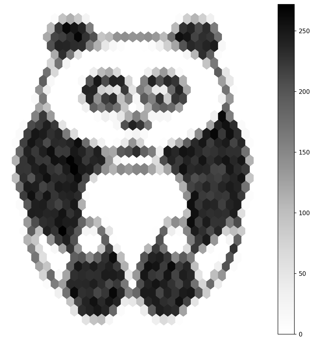

Core concepts

Concept 1 — From pixel grid to long-format DataFrame

The hexbin renderer wants a list of (x, y) points, not a 2D image. The cleanest way to turn an image into that list is the unstack + reset_index pandas idiom:

df = pd.DataFrame(inverted)           # rows = y, columns = x
df = df.unstack()                     # MultiIndex Series: (x, y) → intensity
df = df[df > 0].reset_index()         # drop zeros, flatten to columns
df.columns = ['x', 'y', 'intensity']

• pd.DataFrame(inverted) treats the NumPy 2D array as a table; row index becomes y, column index becomes x.
• .unstack() turns the table into a Series with a two-level index — one level per axis.
• df[df > 0] filters out the background pixels (originally white; inverted to zero).
• .reset_index() promotes the two index levels into ordinary columns.

The output is the long-format table hexbin wants: one row per surviving pixel, three columns named x, y, intensity [3].

Concept 2 — Sampling for an impressionist density

Plotting every surviving pixel would faithfully reconstruct the image; sampling some of them is what makes the output feel like a mosaic rather than a copy:

sample = df.sample(len(df) // 4, random_state=0)   # 25% of the pixels

Sampling does two things at once. It cuts plotting time (millions of points become a few hundred thousand), and it introduces visual stochasticity — the hex cells now reflect a random subset of the source, so they speak of density rather than coverage. The artistic move is to undersample heavily; the analytic move is to keep more of the data.

The random_state=0 argument fixes the random seed so the output is reproducible. Drop it and every run produces a slightly different mosaic.

Concept 3 — gridsize is the abstraction knob

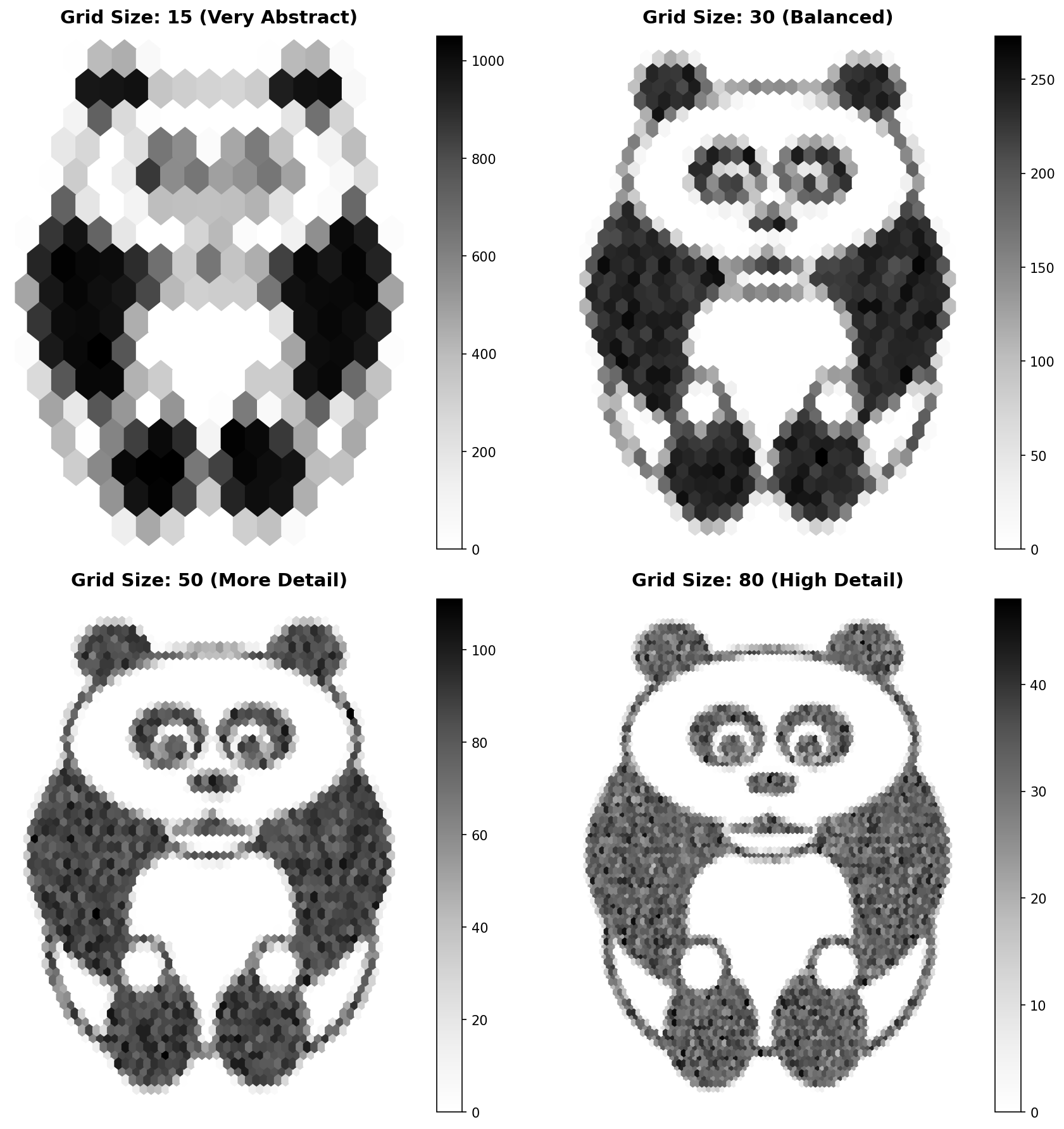
A gridsize=30 hexbin lays down 30 hexagons across the x-axis. Smaller values give bigger hexagons (more abstract); larger values give smaller hexagons (more detail). The choice is almost entirely artistic [4]:

• gridsize=15 — large hexes; the picture reads as a few abstract blobs.
• gridsize=30 — middle ground; subject is recognisable.
• gridsize=60 — small hexes; the picture starts to look like the original through frosted glass.

Exercises

Three exercises in Execute → Modify → Create order: run the hexpanda, swap gridsize and cmap, then build a hexbin from a procedural gradient.

sample.plot.hexbin(x='x', y='y', gridsize=60, cmap='Greys', ax=ax)

sample.plot.hexbin(x='x', y='y', gridsize=15, cmap='Greys', ax=ax)

sample.plot.hexbin(x='x', y='y', gridsize=30, cmap='plasma', ax=ax)

import pandas as pd
import matplotlib.pyplot as plt
import numpy as np

H, W = 200, 200

# TODO 1: build a 2D gradient where intensity = row + col,
#         scaled to 0..255 (uint8). Use np.indices for the (row, col) grid.

# TODO 2: convert to the long DataFrame using the same unstack + reset_index pipeline.

# TODO 3: sample ~50% of the pixels and plot.hexbin with gridsize=25, cmap='viridis'.

plt.savefig('gradient_hexbin.png', bbox_inches='tight', dpi=120)

row, col = np.indices((H, W))
gradient = ((row + col) / ((H - 1) + (W - 1)) * 255).astype(np.uint8)

df = pd.DataFrame(gradient).unstack().reset_index()
df.columns = ['x', 'y', 'intensity']
df['y'] = -df['y']

import pandas as pd
import matplotlib.pyplot as plt
import numpy as np

H, W = 200, 200

row, col = np.indices((H, W))
gradient = ((row + col) / ((H - 1) + (W - 1)) * 255).astype(np.uint8)

df = pd.DataFrame(gradient).unstack().reset_index()
df.columns = ['x', 'y', 'intensity']
df['y'] = -df['y']

sample = df.sample(len(df) // 2, random_state=42)

fig, ax = plt.subplots(figsize=(8, 8))
sample.plot.hexbin(x='x', y='y', gridsize=25, cmap='viridis', ax=ax)
ax.set_aspect('equal'); ax.axis('off')
plt.savefig('gradient_hexbin.png', bbox_inches='tight', dpi=120)

Downloads

Summary

Common pitfalls to avoid

• Skipping the inversion — bright pixels dominate; the subject vanishes.
• Forgetting df['y'] = -df['y'] — the output is upside-down because matplotlib’s y-axis points up while image y-axis points down.
• Calling df.sample(N) with N > len(df) — pandas raises ValueError. Use min(N, len(df)) or a fraction.
• Choosing a colormap that is hard for colourblind viewers — viridis, plasma, cividis are perceptually uniform and safe; Greys is always fine.
• gridsize too small (single-digit) — the hexagons swallow the entire image and the output is just a few coloured blobs.

References

- [1] Carr, D. B., Littlefield, R. J., Nicholson, W. L., & Littlefield, J. S. (1987). Scatterplot matrix techniques for large N. Journal of the American Statistical Association, 82(398), 424–436. doi:10.2307/2289444
- [2] Hunter, J. D. (2007). Matplotlib: A 2D graphics environment. Computing in Science & Engineering, 9(3), 90–95. doi:10.1109/MCSE.2007.55
- [3] McKinney, W. (2010). Data structures for statistical computing in Python. Proceedings of the 9th Python in Science Conference, 51–56.
- [4] Wilkinson, L. (2005). The Grammar of Graphics (2nd ed.). Springer.
- [5] Hales, T. C. (2001). The honeycomb conjecture. Discrete & Computational Geometry, 25(1), 1–22. doi:10.1007/s004540010071
- [6] Harris, C. R., Millman, K. J., van der Walt, S. J., et al. (2020). Array programming with NumPy. Nature, 585, 357–362. doi:10.1038/s41586-020-2649-2