3.3.1 Warhol Pop Art

Overview

Andy Warhol’s Marilyn Diptych (1962) showed the same photographic image fifty times, with different ink colours per silkscreen pass. The radical idea was treating the colour palette itself as a variable of the work, not a fixed property of the subject [1]. In NumPy this collapses to one operation — channel permutation — image[:, :, [2, 0, 1]] reorders the colour axis without touching the pixel values. Six permutations of three channels give six instantly different palettes, all from a single source array. Lay four of them in a 2×2 grid and you have a Warhol pastiche in about ten lines of code [2].

Learning objectives

1. Read image[:, :, [2, 0, 1]] as a channel permutation — same pixels, reordered RGB axes.
2. List the six permutations of three channels and predict the rough colour effect of each.
3. Build a 2×2 grid composition with either a pre-allocated canvas plus slice assignment, or np.vstack/np.hstack.
4. Add a configurable gap between panels by sizing the canvas with 2*W + gap and shifting the second column.

Quick start — a 2×2 Warhol grid

import numpy as np
from PIL import Image

H, W = 200, 200

# A radial sinusoid source — three channels phase-offset
y, x = np.ogrid[:H, :W]
cx, cy = W // 2, H // 2
dist = np.sqrt((x - cx) ** 2 + (y - cy) ** 2)

source = np.zeros((H, W, 3), dtype=np.uint8)
source[..., 0] = (128 + 127 * np.sin(dist * 0.1)        ).astype(np.uint8)
source[..., 1] = (128 + 127 * np.sin(dist * 0.1 + 2)    ).astype(np.uint8)
source[..., 2] = (128 + 127 * np.sin(dist * 0.1 + 4)    ).astype(np.uint8)

# Four different channel permutations placed in a 2×2 canvas
canvas = np.zeros((H * 2, W * 2, 3), dtype=np.uint8)
canvas[0:H,  0:W ] = source[:, :, [0, 1, 2]]   # original
canvas[0:H,  W: ] = source[:, :, [1, 2, 0]]   # rotate left:  RGB → GBR
canvas[H:,   0:W ] = source[:, :, [2, 0, 1]]   # rotate right: RGB → BRG
canvas[H:,   W: ] = source[:, :, [0, 2, 1]]   # swap G ↔ B

Image.fromarray(canvas).save('simple_warhol.png')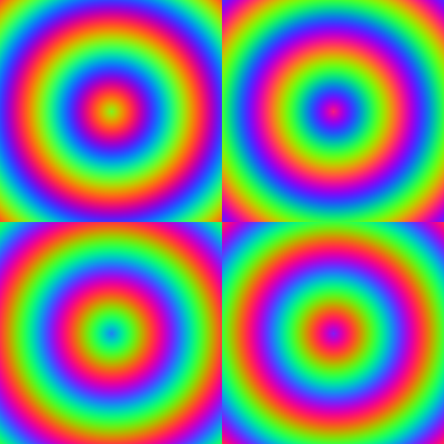

Core concepts

Concept 1 — Channel permutation

A (H, W, 3) array’s last axis is the colour axis. NumPy’s advanced indexing lets you reorder it with a list:

image[:, :, [2, 0, 1]]
# row : keep all
# col : keep all
# chn : reorder — channel 2 first, then 0, then 1

This does not change pixel values. It changes which value the renderer treats as red, which as green, which as blue. Three channels have 3! = 6 orderings:

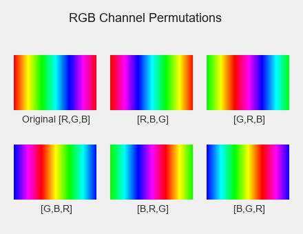
The R↔B swap is the most jarring because it inverts the warm/cool relationship — orange becomes blue, red becomes cyan. Single-pair swaps are gentler than rotations because they only move two values, leaving the third one anchored in place.

Concept 2 — Why this is a Warhol effect

Warhol’s silkscreen process printed each colour separately, on its own pass through the press. By changing which ink loaded into which channel, he produced his series — fifty Marilyns, the Soup Cans, the Brillo Boxes [3]. The art is in the systematic variation, not the individual frame: the viewer’s eye reads them all together and the palette becomes the subject.

The same systematic-variation move is what makes channel permutation feel like a Warhol effect. You are not retouching colour; you are exposing one source image through every possible RGB filter and arranging the results in a grid. The grid composition is what cues the eye to compare, exactly like the gallery wall of Marilyns.

Concept 3 — Grid composition

Two NumPy idioms put N panels into one image. Both produce the same result.

Pre-allocated canvas, slice assignment.

canvas = np.zeros((H * 2, W * 2, 3), dtype=np.uint8)
canvas[0:H,  0:W ] = panel_a
canvas[0:H,  W:  ] = panel_b
canvas[H:,   0:W ] = panel_c
canvas[H:,   W:  ] = panel_d

Reads explicitly: put A in the top-left quadrant. Easy to add a gap (canvas[0:H, W+gap:]) and easy to extend to non-uniform grids.

Stack with hstack / vstack.

top = np.hstack([panel_a, panel_b])
bot = np.hstack([panel_c, panel_d])
canvas = np.vstack([top, bot])

Reads as paste them in row-major order. Shorter for regular grids; awkward when you want gaps because you have to construct gutter rows and columns by hand.

The two methods are interchangeable for this lesson. Pick the one whose intent matches yours.

Exercises

Three exercises in Execute → Modify → Create order: run a six-panel grid, swap permutations, then build a 2×2 from your own source image.

EXECUTE I.

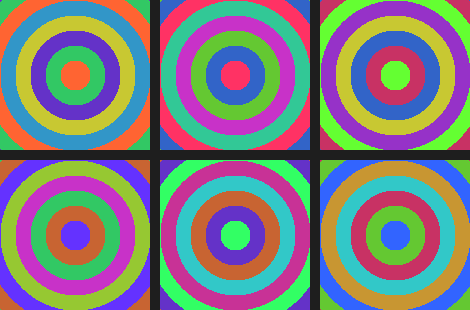
Run all six permutations

Run warhol_variations.py from the downloads. It generates a 2×3 grid showing all six permutations of a concentric-ring source.

Reflection questions

• Which permutation produces the most dramatic colour shift from the original?
• Why do [0, 2, 1] (swap G↔B) and [1, 0, 2] (swap R↔G) look more similar to each other than to [1, 2, 0] (rotate left)?
• Which variation feels most “pop-art” to you, and what makes it read that way?

Answers

Most dramatic — [2, 1, 0] (swap R↔B) usually wins. It exchanges the two channels that humans associate with warm/cool, so the perceived temperature of every pixel flips: orange→blue, yellow→teal, magenta→cyan.

Similar swap pairs — both [0, 2, 1] and [1, 0, 2] leave one channel in place. Rotations like [1, 2, 0] move all three channels at once, which is a bigger perceptual shift even when no individual swap is more extreme than R↔B.

Pop-art feel — taste varies, but the rotations ([1, 2, 0] and [2, 0, 1]) tend to produce the unusual-but-harmonious palettes that the silkscreen tradition trades on. Single swaps can look like Photoshop accidents; rotations look like intent.

canvas[0:H, W:] = source[:, :, [2, 1, 0]]

canvas[H:, 0:W] = source[:, :, [1, 0, 2]]

gap = 5
canvas = np.zeros((H * 2 + gap, W * 2 + gap, 3), dtype=np.uint8)

canvas[0:H,     0:W       ] = source[:, :, [0, 1, 2]]
canvas[0:H,     W + gap:  ] = source[:, :, [2, 1, 0]]
canvas[H + gap:, 0:W       ] = source[:, :, [1, 0, 2]]
canvas[H + gap:, W + gap:  ] = source[:, :, [0, 2, 1]]

CREATE III.

Your own 2×2 with mixed shapes

Build a 2×2 Warhol grid from your own source image. The source should contain at least two visually distinct regions — for example a coloured circle on a striped background — so the permutations produce instantly readable colour shifts.

python · exercise3_starter.py Copy

import numpy as np
from PIL import Image

H, W = 200, 200
source = np.zeros((H, W, 3), dtype=np.uint8)

# Background: diagonal three-colour stripes
y, x = np.ogrid[:H, :W]
stripe = ((x + y) // 20 % 3)
source[(stripe == 0)[0]] = [50, 100, 200]    # ← careful, stripe is broadcast
source[(stripe == 1)[0]] = [100, 200, 100]
source[(stripe == 2)[0]] = [200, 80, 150]

# Orange disc on top
disc = (x - W // 2) ** 2 + (y - H // 2) ** 2 < 60 ** 2
source[disc] = [255, 150, 50]

# TODO 1: build the (H*2, W*2, 3) canvas.
# TODO 2: pick three permutations besides the original and place them in the
#         four quadrants. At least one should be a rotation; at least one a swap.

Image.fromarray(canvas).save('my_warhol.png')

Hint 1 — fix the broadcasting trap

(stripe == 0) produces an (H, W) boolean — source[stripe == 0] = [...] is the cleaner form. The starter’s [0] slice is a red herring; remove it:

source[stripe == 0] = [50, 100, 200]
source[stripe == 1] = [100, 200, 100]
source[stripe == 2] = [200, 80, 150]

Hint 2 — pick three permutations

A balanced choice: one rotation, one R↔B swap, one G↔B swap:

canvas[0:H,  0:W ] = source[:, :, [0, 1, 2]]
canvas[0:H,  W: ] = source[:, :, [1, 2, 0]]   # rotation
canvas[H:,   0:W ] = source[:, :, [2, 1, 0]]   # warm/cool flip
canvas[H:,   W: ] = source[:, :, [0, 2, 1]]   # subtle swap

Complete solution

python · exercise3_solution.py Copy

import numpy as np
from PIL import Image

H, W = 200, 200
source = np.zeros((H, W, 3), dtype=np.uint8)

y, x = np.ogrid[:H, :W]
stripe = (x + y) // 20 % 3
source[stripe == 0] = [50, 100, 200]
source[stripe == 1] = [100, 200, 100]
source[stripe == 2] = [200, 80, 150]

disc = (x - W // 2) ** 2 + (y - H // 2) ** 2 < 60 ** 2
source[disc] = [255, 150, 50]

canvas = np.zeros((H * 2, W * 2, 3), dtype=np.uint8)
canvas[0:H,  0:W ] = source[:, :, [0, 1, 2]]
canvas[0:H,  W: ] = source[:, :, [1, 2, 0]]
canvas[H:,   0:W ] = source[:, :, [2, 0, 1]]
canvas[H:,   W: ] = source[:, :, [2, 1, 0]]

Image.fromarray(canvas).save('my_warhol.png')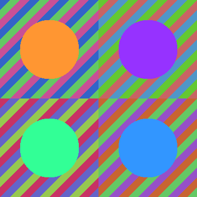

How it works:

• The source builds two layers — diagonal stripes from (x + y) // 20, then an orange disc on top via a circular mask.
• Each quadrant is source[:, :, [perm]] — same pixels, different colour axis order.
• The 2×2 canvas + slice assignment is the most readable layout for a regular grid; np.vstack(np.hstack(...)) is the alternative if you prefer concatenation.

Make it your own

• Combine permutation with a per-quadrant scalar multiply — canvas[0:H, 0:W] = source[:, :, [0, 1, 2]] // 2 for a “Marilyn fading” effect.
• Render a 3×3 (np.zeros((3*H, 3*W, 3))) with all six permutations plus three horizontal-flipped extras: source[:, ::-1, perm].
• Use one of your own photos as the source instead of the procedural pattern — the channel-permutation effect is wildest on portraits.

Downloads

Summary

Common pitfalls to avoid

• Confusing [2, 0, 1] (channel order) with [2, 0, 1, ...] (full array index) — the former is the third axis only.
• Treating channel permutation as colour correction — it is not gamma, hue rotation, or colour balance; it just reorders.
• Calculating canvas dimensions with width * 2 when you meant height * 2 — NumPy shape is (H, W, 3), easy to flip mentally.
• Using np.concatenate(axis=0) instead of np.vstack — equivalent in 2D and 3D but vstack is more readable.
• Forgetting that the second slice endpoint is exclusive: 0:H covers pixels 0..H-1, not 0..H.

References

- [1] Warhol, A. (1975). The Philosophy of Andy Warhol (From A to B and Back Again). Harcourt Brace Jovanovich.
- [2] Harris, C. R., Millman, K. J., van der Walt, S. J., et al. (2020). Array programming with NumPy. Nature, 585, 357–362. doi:10.1038/s41586-020-2649-2
- [3] Foster, H. (2012). The First Pop Age: Painting and Subjectivity in the Art of Hamilton, Lichtenstein, Warhol, Richter, and Ruscha. Princeton University Press.
- [4] Tate Modern. (2024). Andy Warhol: Marilyn Diptych, 1962. Tate Collection. tate.org.uk
- [5] Albers, J. (2013). Interaction of Color (50th anniversary ed.). Yale University Press.
- [6] Gonzalez, R. C., & Woods, R. E. (2018). Digital Image Processing (4th ed.). Pearson.